Hashing in Data Structures

Introduction to Hashing

Hashing in data structures is the technique or practice of employing a hash function to map keys and values into a hash table. It is done so that elements can be accessed more quickly. The efficiency of mapping is determined by the effectiveness of the hash function used.

Let's say a hash function H(x) converts the value x in an Array to the index x % 10. For example, if the list of values is [11, 12, 13, 14, 15], it will be put in the array or Hash table at locations 1, 2, 3, 4, and 5 respectively.

A hash table is a data structure that holds information in an associative manner. Data access becomes very speedy if we know the index of the needed data. As a result, regardless of data size, it becomes a data structure with incredibly fast insertion and search operations. Hash Tables are arrays that use the hash technique to generate an index from which an element can be entered or located.

Core Concepts of Hashing

Hashing revolves around a few key ideas that work together to provide its signature speed and efficiency.

What is hashing? How does it work?

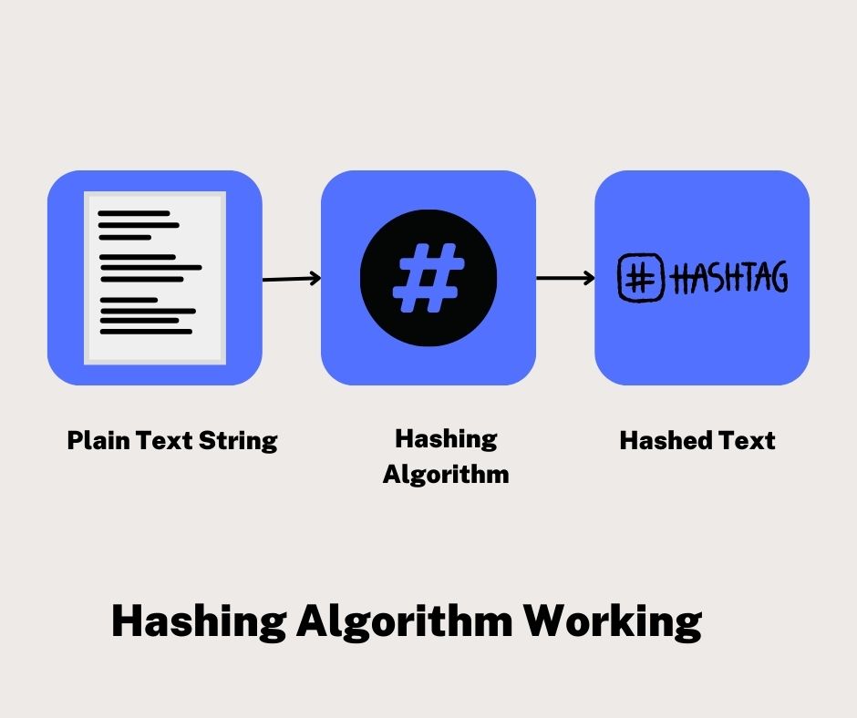
Hashing is the process of converting a given key into a smaller, fixed-size value that can be retrieved in O(1) time on average. This is accomplished by using a function or technique known as a hash function to translate data into an encrypted or simplified representative value known as a "hash code" or "hash." This hash is then used as an index to narrow down search criteria and swiftly retrieve data.

Let's look at an example. Suppose we want to map a list of countries to their capital cities. We can use a hash function to do this. For simplicity, let's say our hash function is to take the length of the string key.

When we apply the hash function (string length), we get an index. We then store the key and value at that index. 'Cuba' has a length of 4, so it goes into index 4. 'Spain' has a length of 5, so it goes into index 5, and so on.

This simple example has flaws (e.g., what if two keys have the same length?), which leads to the concept of collision handling, but it illustrates the basic principle of mapping a key to an index for fast lookups.

Are Hashing algorithms secure?

It depends on the type. Secure Hashing Algorithms (SHAs) are a subset of hashing algorithms specifically designed for security. These are also known as cryptographic hashing algorithms.

Key properties of cryptographic hash functions include:

• One-way: It is computationally infeasible to reverse the function and find the original input from the hash output.
• Collision Resistance: It is extremely difficult to find two different inputs that produce the same hash output.

Algorithms like SHA-256 are considered secure and are widely used for password storage, digital signatures, and blockchain technology. In contrast, non-cryptographic hash functions used in data structures (like hash tables) prioritize speed and uniform distribution over security.

Who invented Hashing?

Hans Peter Luhn, a computer scientist at IBM, is credited with the invention of hashing. In a 1953 internal IBM memorandum, he proposed the idea. His work was later formalized, and he presented it at a conference in 1958.

How does Hashing work?

Hashing primarily works by using a function called a "hash function" to convert data of any arbitrary size to a fixed-size value and storing it in a data structure called a "hash table" at the value produced by hash functions. Hash codes, digests, hash values, and hashes are all terms for the values returned by this function.

Why can't the results of hashing be reverted back to the original input?

This is a key feature of cryptographic hash functions, which are designed to be "one-way". The process is irreversible for two main reasons:

1. Loss of Information: Hash functions map an input of potentially infinite size (e.g., any text document) to an output of a fixed, smaller size (e.g., 256 bits for SHA-256). This means many different inputs will map to the same output (a collision). Since information is lost in this mapping, you cannot definitively determine the original input from the output alone.
2. Computational Difficulty: The mathematical operations within cryptographic hash functions are designed to be extremely difficult and computationally expensive to reverse. This property, known as "pre-image resistance," ensures that even if you have the hash, you can't find the original message without trying every possible input, which is infeasible.

When is it not advisable to use Hashing/Hash Tables?

While hashing provides excellent average-case performance, it's not always the best choice:

• Small Data Sets: For very small amounts of data, the overhead of a hash table (extra memory, hash function computation) can be greater than the benefit. A simple array or list might be faster and more memory-efficient.
• Ordered Data Requirement: Hash tables do not maintain data in any specific order (like sorted order). If you need to iterate through elements in a sorted manner or find the minimum/maximum key, a balanced binary search tree (like a Red-Black Tree) or a sorted array would be a better data structure.
• Worst-Case Performance Concerns: Although rare with a good hash function, the worst-case time complexity for hash table operations is O(n). If your application requires guaranteed O(log n) performance even in the worst case, a self-balancing binary search tree is a safer choice.

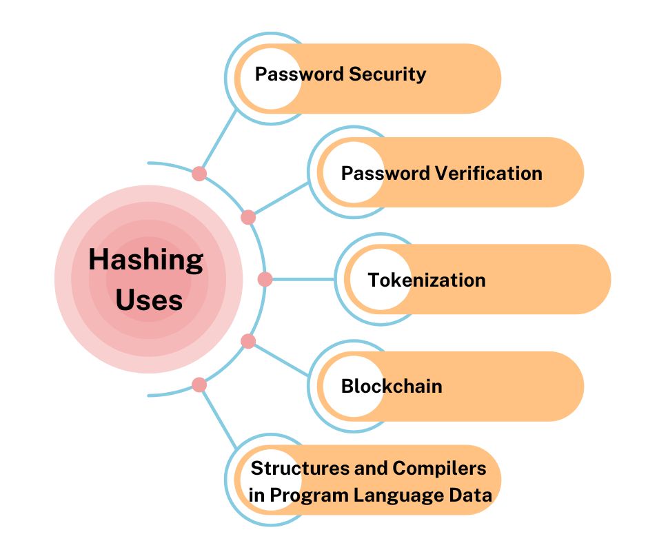
Where is Hashing used?

Hashing is a ubiquitous technique in computer science with a vast range of applications:

• Database Indexing: To quickly locate records in a database without scanning the entire table.
• Caching: To store and retrieve frequently accessed data in memory for rapid access.
• Password Security: Storing password hashes instead of plain text passwords to protect user credentials.
• Compiler Symbol Tables: To efficiently store and look up variables, functions, and keywords during compilation.
• Associative Arrays (Dictionaries/Maps): Implementing key-value data structures in programming languages like Python's `dict` and Java's `HashMap`.
• Blockchain: Cryptographic hashing is fundamental to linking blocks securely and ensuring the integrity of the ledger.
• File Integrity Checks: Using hashes (like MD5 or SHA-256) to verify that a downloaded file has not been corrupted or tampered with.

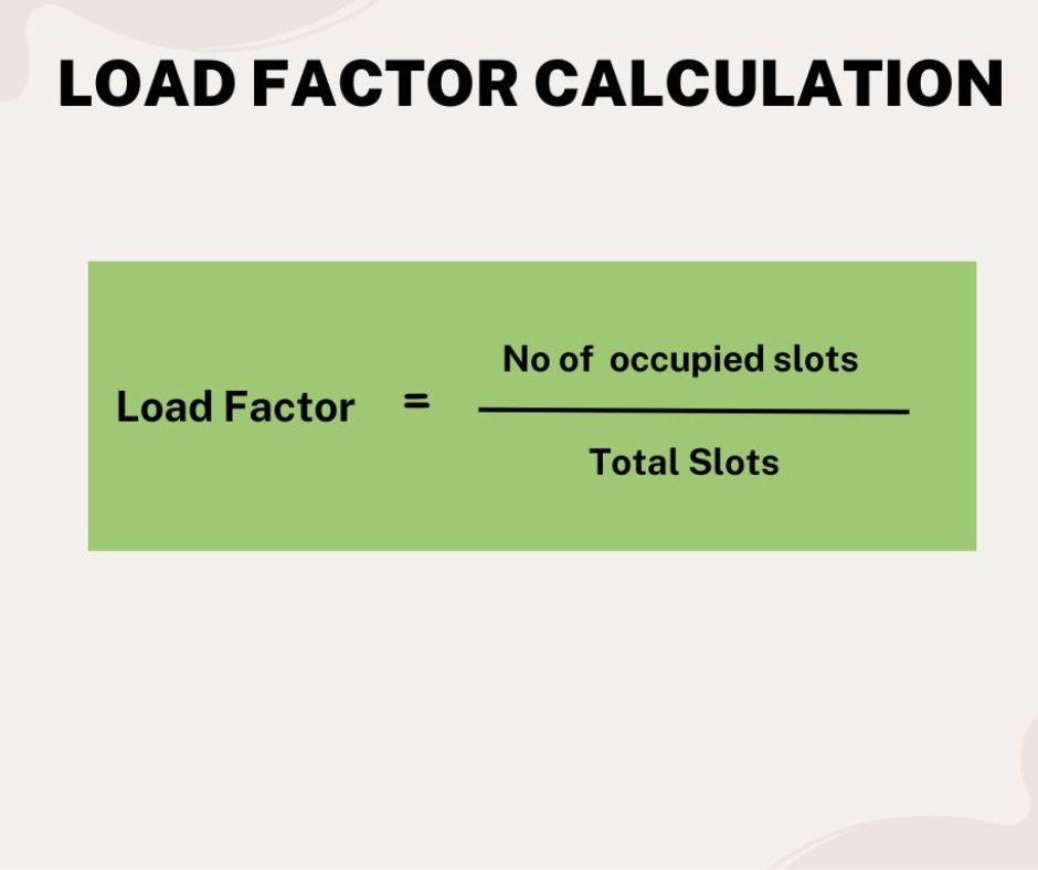
What is a Load Factor?

The load factor (often denoted by alpha, α) is a critical metric for a hash table that measures how full it is. It is calculated as:

α = (Number of elements in the table) / (Size of the hash table)

For example, if a hash table has a size of 1000 and contains 500 elements, its load factor is 500 / 1000 = 0.5.

The load factor represents a trade-off:

• A high load factor means the table is dense, which saves space but increases the probability of collisions. This can degrade performance, making lookups slower.
• A low load factor means the table is sparse, which reduces collisions and improves performance but wastes memory.

Many hash table implementations (like Java's `HashMap`) automatically resize the table (a process called rehashing) when the load factor exceeds a certain threshold (commonly 0.75) to maintain optimal performance.

What are the Basic Operations that can be performed on a hash map?

The three fundamental operations for any hash map or hash table are:

1. Insert: Adds a new key-value pair to the table. This involves calculating the key's hash to find the correct bucket and then adding the element. Average time: O(1).
2. Search/Lookup: Retrieves the value associated with a given key. It calculates the key's hash to find the bucket and then searches within that bucket for the key. Average time: O(1).
3. Delete: Removes a key-value pair from the table. It finds the element using the same process as search and then removes it. Average time: O(1).

What is a Hash Method?

A "Hash Method" is another term for a hash function. It's the algorithm that takes an input key and computes a hash code, which is then typically mapped to an index in the hash table array. For example, a simple hash method for an integer key `k` and a table of size `s` could be:

int hashCode(int key, int tableSize) {
    return key % tableSize;
}

Applications of Hashing

Hashing's irreversibility and constant time access properties have found applications in a variety of domains. The following are some examples:

• Security and Password Verification: The "one-way" nature of cryptographic hash functions is crucial. When you sign up for a service, your password is not stored directly. Instead, its hash is stored. When you log in, the system hashes the password you enter and compares it to the stored hash. This means even if an attacker steals the database, they don't get the actual passwords.
• Data Structures: Core to programming languages, such as `HashMap` in Java, `unordered_map` in C++, and `dict` in Python.
• Compiler Development: Compilers use hash tables to manage symbol tables, which store keywords, variables, and function names for fast lookups during the compilation process.
• Message Digests: Cryptographic hashes are used to ensure file integrity. When you download a large file, a hash (like SHA-256) is often provided. You can compute the hash of your downloaded file and compare it to the provided one. If they match, the file is intact and authentic.
• Other applications include the Rabin-Karp algorithm for string searching, generating git commit IDs, caching data in web servers, blockchain technology, and much more.

What is a DataItem?

In the context of implementing a hash table from scratch, a `DataItem` is a simple structure or class used to hold the key-value pair together as a single unit. It represents the element that will be stored in the hash table.

struct DataItem {
    int key;
    std::string value; // Example value type
};

Search Operation Details

To find an element with a given key:

1. Calculate the hash code of the key to get the initial bucket index.
2. Go to that index in the hash table array.
3. If using Separate Chaining: Traverse the linked list at that index, comparing the key of each node with the target key. If found, return the value. If the end of the list is reached, the key is not in the table.
4. If using Open Addressing (like Linear Probing): Check the element at the index. If it's the correct key, return the value. If the slot is empty, the key is not in the table. If the slot is occupied by a different key, move to the next slot according to the probing sequence (e.g., index + 1) and repeat until the key is found or an empty slot is encountered.

Insertion Operation Details

To insert a new key-value pair:

1. Calculate the hash code of the key to determine the target bucket index.
2. Go to that index in the hash table array.
3. If using Separate Chaining: Before adding, it's good practice to traverse the linked list to see if the key already exists. If it does, you can update the value. If not, add the new key-value pair as a new node to the list (often at the beginning for O(1) insertion).
4. If using Open Addressing: Go to the target index. If the slot is empty or marked as "deleted," insert the new element there. If it's occupied, follow the probing sequence to find the next available empty slot and place the element there.
5. After insertion, check if the load factor has exceeded its threshold. If so, perform a rehashing operation.

Deletion Operation Details

To delete a key-value pair:

1. First, perform a search operation to locate the element.
2. If using Separate Chaining: Once the node with the key is found in the linked list, remove it using standard linked list deletion logic.
3. If using Open Addressing: This is trickier. You cannot simply empty the slot, as it would break the "probe chain" for other elements that might have collided and been placed further down the sequence. Instead of emptying the slot, you must mark it with a special "deleted" or "tombstone" marker. This tells the search operation to keep probing past this slot, while the insert operation knows it can overwrite this slot with a new element.

What is a Hash Function?

A hash function is a fixed process that converts an input key of arbitrary size into a fixed-size output, known as a hash value or hash code. This hash code is then used as an index into the hash table.

The properties of a good hash function for a data structure are:

1. Efficiency: It should be fast to compute.
2. Uniform Distribution: It should map keys as evenly as possible across the hash table's slots to minimize collisions. Each table position should be equally likely for any given key.

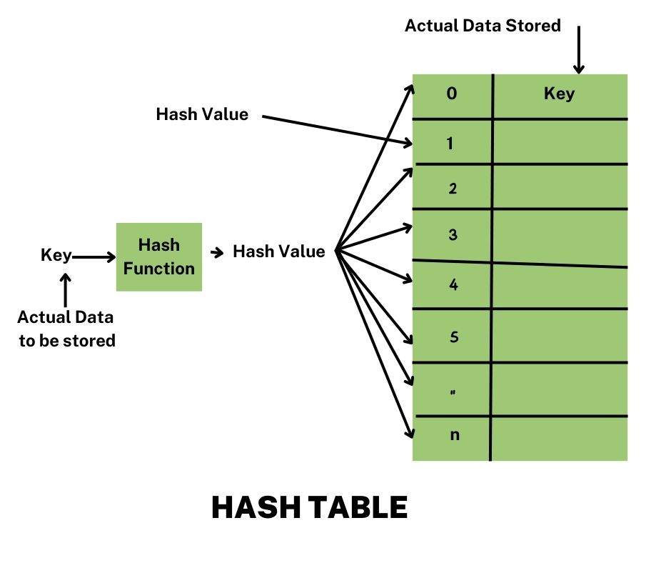
What is a Hash Table?

A hash table, also known as a hash map, is a data structure that implements an associative array abstract data type, a structure that can map keys to values. A hash table uses a hash function to compute an index, also called a hash code, into an array of buckets or slots, from which the desired value can be found.

It is one of the most efficient data structures for lookup, insertion, and deletion operations, providing an average time complexity of O(1) for these actions.

Collision Handling

A collision occurs when a hash function maps two or more different keys to the same index in the hash table. Since it's impossible to store multiple items in the same slot, we need strategies to handle these collisions.

The two main strategies for collision resolution are:

1. Separate Chaining: In this method, each bucket in the hash table does not store the element itself, but rather a pointer to another data structure, typically a linked list. All keys that hash to the same index are stored in the linked list of that bucket.
2. Open Addressing: In this method, all elements are stored directly within the hash table array itself. When a collision occurs, the algorithm systematically probes the table to find an alternative, empty slot to store the collided key.

Linear Probing

Linear probing is a type of Open Addressing. When a collision occurs (i.e., we try to insert a key into a slot that is already occupied), we simply check the next slot in the table.

The probe sequence is `h(k), h(k)+1, h(k)+2, ...`, wrapping around the table if necessary. We continue checking sequentially until an empty slot is found.

Disadvantage: Linear probing suffers from a problem called primary clustering, where long runs of occupied slots build up, increasing the average search time. As one cluster gets bigger, it becomes more likely to be hit, making it grow even larger.

Double Hashing

Double hashing is another, more sophisticated, Open Addressing technique designed to mitigate the clustering problem of linear probing. It uses two different hash functions:

• `h1(k)`: The primary hash function that determines the initial probe location.
• `h2(k)`: A secondary hash function that determines the step size for the probe sequence.

The probe sequence is `(h1(k) + i * h2(k)) % tableSize`, for `i = 0, 1, 2, ...`. Because the step size `h2(k)` depends on the key, different keys that initially collide will likely have different probe sequences, which helps to spread elements more uniformly across the table and avoid primary clustering.

Quadratic Probing

Quadratic probing is an open addressing technique that aims to solve the primary clustering issue of linear probing. Instead of a linear step size, it uses a quadratic polynomial to determine the probe sequence.

The probe sequence is `(h(k) + c1*i + c2*i^2) % tableSize`, where `c1` and `c2` are constants and `i = 0, 1, 2, ...`.

While it avoids primary clustering, it can suffer from a milder problem called secondary clustering, where keys that hash to the same initial location will have the exact same probe sequence.

How Hashing Works (Detailed)

The process of using a hash map to store a key-value pair involves two main steps:

1. Hashing the Key: The key is passed to a hash function, which computes an integer hash code from it. This step should be fast and deterministic (the same key always produces the same hash code).
2. Mapping to an Index: The generated hash code is then mapped to a valid index within the hash table's underlying array. A common way to do this is with the modulo operator: `index = hashCode % arraySize`.
3. Handling Collisions: At the calculated index, the system handles the storage. If using Separate Chaining, it adds the new key-value pair to the linked list at that index (after checking for duplicates). If using Open Addressing, it places the pair at the index if empty, or probes for the next available slot if a collision occurs.

Complexity and Load Factor

The time complexity of hash table operations is heavily influenced by the load factor (α).

• Hash Computation: This is generally considered O(1), assuming the key size is bounded.
• Search/Insert/Delete:
  • Average Case: The average number of elements to check in a bucket is proportional to the load factor. If α is kept small (e.g., below 1.0 for separate chaining), the average time complexity is O(1 + α), which simplifies to O(1).
  • Worst Case: In the worst-case scenario, all 'n' elements hash to the same bucket. This turns the hash table into a single linked list, and the time complexity for operations degrades to O(n). A good hash function makes this extremely unlikely.

Rehashing

Rehashing is the process of creating a new, larger hash table and re-inserting all the elements from the old table into the new one. This operation is triggered when the load factor of the current hash table exceeds a certain threshold (e.g., 0.75). The size of the new table is typically double the size of the old one.

Why Rehash?

Rehashing is essential for maintaining the O(1) average time complexity of hash table operations. As more elements are inserted, the load factor increases. A high load factor leads to more collisions, which in turn increases the length of the chains (in Separate Chaining) or the length of probe sequences (in Open Addressing). This degrades performance, pushing the operation time closer to O(n). By resizing the table and redistributing the elements, rehashing keeps the load factor low and ensures that operations remain fast.

How is Rehashing done?

The process of rehashing involves these steps:

1. When the load factor exceeds the threshold, a new, larger array is created (usually double the original size).
2. Iterate through every element in the old hash table.
3. For each element, recalculate its hash code based on the new table size. This will likely result in a different index.
4. Insert the element into its new position in the new, larger table.
5. Once all elements have been moved, the old table is discarded, and the new table becomes the active hash table.

Note that rehashing can be an expensive operation (O(n)), but since it happens infrequently, its cost is "amortized" over many cheap O(1) insertions, so the average insertion time remains O(1).

Advantages of Double Hashing

• It significantly reduces the problem of clustering that affects linear and quadratic probing.
• It produces a more uniform distribution of keys across the hash table.
• Because the probe sequence depends on two independent hash functions, it's one of the most effective collision resolution techniques for open addressing.

Index Mapping Method

"Index Mapping," also known as Trivial Hashing, is the simplest form of hashing. It's used when the keys themselves are small integers that can be directly used as array indices. For example, if you have keys from 0 to 99, you can use an array of size 100, and the hash function is simply `h(key) = key`.

This method is extremely fast (O(1) in the worst case) and has no collisions. However, it's only practical if the range of keys is small and dense, as it would be highly wasteful of space for large or sparse key ranges (e.g., using employee IDs as keys would require a massive, mostly empty array).

Division Method

This is one of the most common and simplest hash functions. The hash code is calculated by taking the remainder of the key divided by the table size.

Formula: `h(key) = key % tableSize`

Important Consideration: The choice of `tableSize` is crucial. For best results, `tableSize` should be a prime number. If the table size is a power of 2 (e.g., 1024), the hash will only depend on the lower bits of the key, which can lead to poor distribution if the keys have patterns in their lower bits. A prime number helps ensure the hash depends on all parts of the key.

Mid-Square Method

The mid-square method is another hash function technique. It involves these steps:

1. Square the key.
2. Extract a certain number of digits from the middle of the result.
3. This middle part becomes the hash index.

For example, if the key is `3101` and we need a 3-digit index:

1. (3101)² = 9616201
2. Extract the middle 3 digits: `616`.
3. The hash index is `616`.

This method often produces a good distribution because most or all digits of the key contribute to the result.

Multiplication Method

The multiplication method for creating a hash function works as follows:

1. Choose a constant `A` such that `0 < A < 1`. A common choice is `A ≈ (√5 - 1) / 2 ≈ 0.6180339887` (the golden ratio conjugate).
2. Multiply the key `k` by `A`: `k * A`.
3. Extract the fractional part of the result: `(k * A) - floor(k * A)`.
4. Multiply this fractional part by the table size `m`.
5. Take the floor of the result to get the final index: `floor(m * (k * A mod 1))`.

A key advantage of this method is that the choice of table size `m` is not critical. It works well for any `m`, though powers of 2 are often chosen for implementation efficiency.

Load Factor (Revisited)

The load factor is the ratio of the number of elements stored in the hash table to the total number of available slots. It's a critical measure of how full the table is.

Load Factor (α) = n / m (where n = number of elements, m = table size)

Maintaining a reasonable load factor (typically below 0.75 or 1.0) is crucial for performance. If the load factor gets too high, the frequency of collisions increases, and the average time for operations degrades. This is why rehashing is performed when the load factor crosses a certain threshold.

Advantages of Separate Chaining

• Simple Implementation: The logic for insertion and deletion is relatively straightforward compared to some open addressing techniques.
• Unlimited Elements: The hash table itself never technically "fills up." You can always add more elements to the chains (though performance degrades).
• Less Sensitive to Load Factor: Performance degrades more gracefully as the load factor grows beyond 1.0.
• Easy Deletion: Deleting an element is simple linked-list node removal, unlike the "tombstone" complexity in open addressing.

Disadvantages of Separate Chaining

• Memory Overhead: Each node in the linked lists requires extra memory to store a pointer to the next node, which can be significant for small data items.
• Poor Cache Performance: The nodes of a linked list can be scattered throughout memory. Traversing a list can lead to frequent cache misses, which is slower than accessing contiguous memory in an array (as is more common in open addressing).
• Worst-Case Degeneration: In the highly unlikely worst-case scenario where all keys hash to the same bucket, the structure degenerates into a single linked list, and all operations become O(n).

Open Addressing

Open addressing is a collision resolution strategy where all elements are stored directly in the hash table array itself. When a new key hashes to a slot that is already occupied, the algorithm probes for an alternative empty slot according to a determined sequence.

Key aspects of open addressing:

• The table size must be at least as large as the number of keys.
• The load factor (α) must always be less than or equal to 1.
• Deletion requires a special "tombstone" marker to avoid breaking probe chains.
• Common probing techniques include Linear Probing, Quadratic Probing, and Double Hashing.

Open addressing generally has better cache performance than separate chaining because elements are stored contiguously in an array.

Implementation Examples

C++ Implementation

Here's a basic hash table implementation in C++ using separate chaining.

#include <iostream>
#include <vector>
#include <list>
#include <string>

class HashTable {
private:
    int size;
    std::vector>> table;

    int hashFunction(int key) {
        return key % size;
    }

public:
    HashTable(int s) : size(s) {
        table.resize(size);
    }

    void insert(int key, std::string value) {
        int index = hashFunction(key);
        for (auto& pair : table[index]) {
            if (pair.first == key) {
                pair.second = value; // Update if key exists
                return;
            }
        }
        table[index].push_back({key, value});
    }

    std::string search(int key) {
        int index = hashFunction(key);
        for (auto const& pair : table[index]) {
            if (pair.first == key) {
                return pair.second;
            }
        }
        return "Not Found";
    }
    
    void remove(int key) {
        int index = hashFunction(key);
        table[index].remove_if([key](const std::pair& pair){
            return pair.first == key;
        });
    }
};

Java Implementation

Java has a built-in `HashMap` class. Here's how you use it.

import java.util.HashMap;
import java.util.Map;

public class HashExample {
    public static void main(String[] args) {
        // Declaration
        Map<String, String> capitalCities = new HashMap<>();

        // Inserting Key-Value pairs
        capitalCities.put("England", "London");
        capitalCities.put("Germany", "Berlin");
        capitalCities.put("India", "New Delhi");

        // Searching a Key
        System.out.println("Capital of England: " + capitalCities.get("England")); // London
        System.out.println("Contains key 'France': " + capitalCities.containsKey("France")); // false

        // Finding Size
        System.out.println("Map size: " + capitalCities.size()); // 3
        
        // Erasing from the Map
        capitalCities.remove("Germany");
        System.out.println("Map after removing Germany: " + capitalCities);
    }
}

Python Implementation

Python's dictionary (`dict`) is its built-in hash map implementation.

# Declaration (creates an empty dictionary)
capital_cities = {}

# Inserting Key-Value pairs
capital_cities["England"] = "London"
capital_cities["Germany"] = "Berlin"
capital_cities["India"] = "New Delhi"

# Searching a Key
print(f"Capital of England: {capital_cities.get('England')}")  # Use .get() to avoid errors for missing keys
print(f"Is 'France' a key? {'France' in capital_cities}")

# Finding Size
print(f"Dictionary size: {len(capital_cities)}")

# Erasing from the Map
if "Germany" in capital_cities:
    del capital_cities["Germany"]

print(f"Dictionary after removing Germany: {capital_cities}")

Frequently Asked Questions