A term that keeps popping up whenever graphs are mentioned is ‘traversal’. But, what exactly is meant by the ‘traversal’ of a graph? To ‘traverse’ a graph is to visit all its vertices. What do you mean ‘visit’? Alright, look at the graph below:

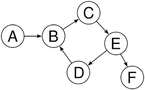
When we say we are visiting the ‘Node A’, we mean that we are focusing on ‘Node A’ and not on the other nodes. While we are focusing on ‘Node A’, we might obtain information from it, print it, or change/update it. When we are done focusing on the ‘Node A’, we move to some other node in the graph and we say that we have traversed the ‘Node A’. Similarly, we traverse the other nodes.

Breadth First Search (BFS) is an algorithm for the traversal of graphs. What this means is that when we implement BFS on a graph, we choose a ‘source’ node and starting from this node, we traverse all other nodes in a well defined manner instead of jumping from one node to another randomly.

Understanding the Breadth-First Search Algorithm with an example

Breadth-First Search algorithm follows a simple, level-based approach to solve a problem. Consider the below binary tree (which is a graph). Our aim is to traverse the graph by using the Breadth-First Search Algorithm.

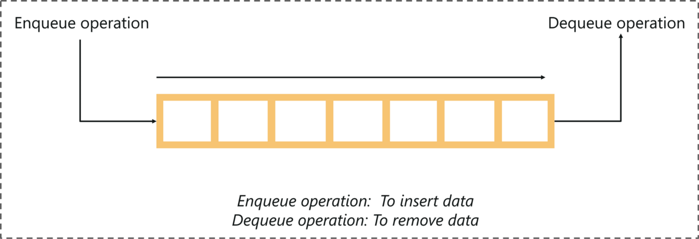
Before we get started, you must be familiar with the main data structure involved in the Breadth-First Search algorithm.

A queue is an abstract data structure that follows the First-In-First-Out methodology (data inserted first will be accessed first). It is open on both ends, where one end is always used to insert data (enqueue) and the other is used to remove data (dequeue).

Now let’s take a look at the steps involved in traversing a graph by using Breadth-First Search:
Step 1: Take an Empty Queue.
Step 2: Select a starting node (visiting a node) and insert it into the Queue.
Step 3: Provided that the Queue is not empty, extract the node from the Queue and insert its child nodes (exploring a node) into the Queue.
Step 4: Print the extracted node.
Don’t worry if you’re confused, we shall understand this with an example.
Take a look at the below graph, we will use the Breadth-First Search algorithm to traverse through the graph.

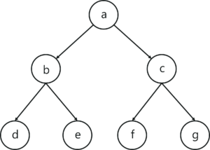
In this case, we’ll assign node ‘a’ as the root node and start traversing downward and follow the steps mentioned above.

Application

Most of the concepts in computer science and real world can be visualized and represented in terms of graph data structure. BFS is one such useful algorithm for solving these problems easily. The architecture of BFS is simple, accurate and robust. It is very seamless as it is guaranteed that the algorithm won’t get caught in an infinite loop.

Shortest Path: In an unweighted graph, the shortest path is the path with least number of edges. With BFS, we always reach a node from given source in shortest possible path. Example: Dijkstra’s Algorithm.

GPS Navigation Systems: BFS is used to find the neighboring locations from a given source location.

Finding Path: We can use BFS to find whether a path exists between two nodes.

Social Networking Websites: We can find number of people within a given distance ‘k’ from a person using BFS.

Implementation in Python

# BFS algorithm in Python


import collections

# BFS algorithm
def bfs(graph, root):

    visited, queue = set(), collections.deque([root])
    visited.add(root)

    while queue:

        # Dequeue a vertex from queue
        vertex = queue.popleft()
        print(str(vertex) + " ", end="")

        # If not visited, mark it as visited, and
        # enqueue it
        for neighbour in graph[vertex]:
            if neighbour not in visited:
                visited.add(neighbour)
                queue.append(neighbour)


if __name__ == '__main__':
    graph = {0: [1, 2], 1: [2], 2: [3], 3: [1, 2]}
    print("Following is Breadth First Traversal: ")
    bfs(graph, 0)

Implementation in C++

// BFS algorithm in C++

#include <iostream>
#include <list>

using namespace std;

class Graph {
  int numVertices;
  list<int>* adjLists;
  bool* visited;

   public:
  Graph(int vertices);
  void addEdge(int src, int dest);
  void BFS(int startVertex);
};

// Create a graph with given vertices,
// and maintain an adjacency list
Graph::Graph(int vertices) {
  numVertices = vertices;
  adjLists = new list<int>[vertices];
}

// Add edges to the graph
void Graph::addEdge(int src, int dest) {
  adjLists[src].push_back(dest);
  adjLists[dest].push_back(src);
}

// BFS algorithm
void Graph::BFS(int startVertex) {
  visited = new bool[numVertices];
  for (int i = 0; i < numVertices; i++)
    visited[i] = false;

  list<int> queue;

  visited[startVertex] = true;
  queue.push_back(startVertex);

  list<int>::iterator i;

  while (!queue.empty()) {
    int currVertex = queue.front();
    cout << "Visited " << currVertex << " ";
    queue.pop_front();

    for (i = adjLists[currVertex].begin(); i != adjLists[currVertex].end(); ++i) {
      int adjVertex = *i;
      if (!visited[adjVertex]) {
        visited[adjVertex] = true;
        queue.push_back(adjVertex);
      }
    }
  }
}

int main() {
  Graph g(4);
  g.addEdge(0, 1);
  g.addEdge(0, 2);
  g.addEdge(1, 2);
  g.addEdge(2, 0);
  g.addEdge(2, 3);
  g.addEdge(3, 3);

  g.BFS(2);

  return 0;
}

Time & Space Complexity Analysis

The time complexity of the BFS algorithm is represented in the form of O(V + E), where V is the number of nodes and E is the number of edges.
The space complexity of the algorithm is O(V).

With this article at Logicmojo, you must have the complete idea of analyzing BFS algorithm.

Good Luck & Happy Learning!!