Introduction

The ability of artificial intelligence to close the gap between human and computer skills has been growing dramatically. Both professionals and amateurs focus on many facets of the field to achieve great results. The field of computer vision is one of several such disciplines.

The goal of this field is to give robots the ability to see the environment similarly as humans do and to use that understanding for a variety of activities, including image and video recognition, image analysis, media recreation, recommendation systems, natural language processing, etc. With time, one particular algorithm—a Convolutional Neural Network—has been developed and optimised, primarily leading to breakthroughs in computer vision with deep learning.

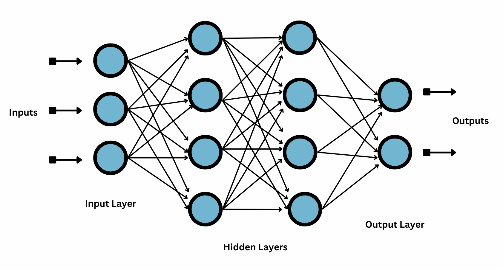
Let's first review the basic concepts of neural networks before delving into the Convolution Neural Network. There are three different sorts of layers in a typical neural network:

1. Input Layer

2. Hidden Layer

3. Output Layer

what is Deep Learning

What is convolutional neural network?

A Convolutional Neural Network (ConvNet/CNN) is a Deep Learning method which can take in such an image as input, give different elements and objects in the image significance (learnable weights and biases), and be capable of distinguishing between them. Comparatively speaking, a ConvNet requires substantially less pre-processing than other classification techniques. ConvNets have the capacity to learn these filters and properties, whereas in primitive techniques filters are hand-engineered.

There are other kinds of neural nets, which are utilised for diverse use cases and data types, while we mainly concentrated on feedforward networks in that article. Recurrent neural networks, for instance, are frequently used for speech and natural language processing, but convolutional neural networks (also known as CNNs or ConvNets) are more frequently employed for classification and computer vision applications. Before CNNs, identifying objects in images required the use of laborious, manual feature extraction techniques.

Convolutional neural networks, on the other hand, now offer a more scalable method for classifying images and recognising objects by using matrix multiplication and other concepts from linear algebra to find patterns in images. However, they can be computationally taxing, necessitating the use of graphics processing units (GPUs) when modelling them.

Learn More️

Understanding Convolutional Neural Network

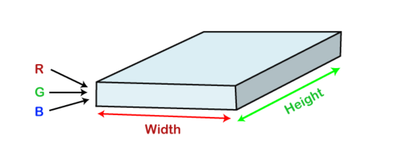
Convolution Neural networks that integrate their parameters are known as covnets. Consider having an image. It can be visualised as a cuboid with its length, breadth (the image's dimension), and height (as images generally have red, green, and blue channels).

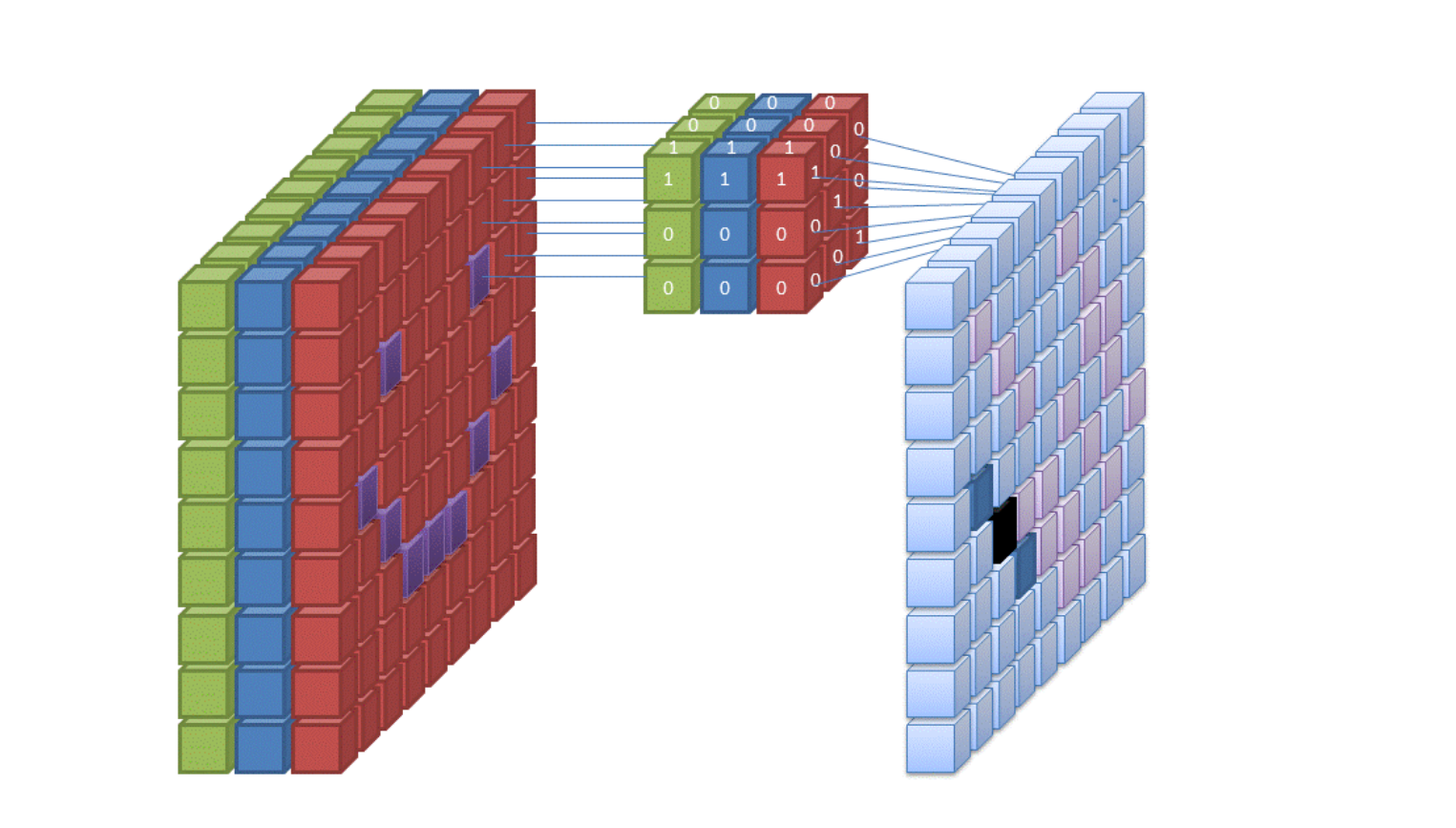
Consider running a small neural network with, say, k outputs on a small portion of this image and representing the results vertically. Move the neural network across the entire image, and a new image with altered width, height, and depth will appear. We now have extra channels, however they are narrower and taller than the original R, G, and B channels. Convolution refers to this process. It will be a normal neural network if the patch size is identical to the image size. This little patch means that there are fewer weights.

It may be represented mathematically as follows:

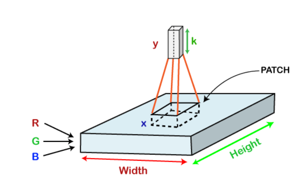
1. The learnable filters included in the convolutional layers have the same tiny width, height, and depth as the input volume being used (if the image is the input layer then probably it would be 3).

2. Imagine that we wish to perform convolution on an image of 34x34x3 of dimensions, allowing for an axax3-sized filter. Any of the above 3, 5, 7, etc., can be an in this case. In relation to the image's size, it must be small.

3. During the forward pass, each filter slides all over the input volume. It slides in discrete steps, referring to each as a stride that, for higher-dimensional images, includes a value of 2 or 3 or 4. Next, it calculates a dot product between the weights of the filter and the patch made from the input volume.

4. As and when we slide our filters, followed by stacking them together to accomplish an output volume to have a similar depth value to that of the number of filters, it will produce a 2-Dimensional output for each filter. The network will then finish learning all the filters.

How do convolutional neural networks work?

Convolutional neural networks outperform other neural networks when given inputs such as images, voice, or audio, for example. There are three main categories of layers in them:

1. Convolutional layer

2. Pooling layer

3. Fully-connected (FC) layer

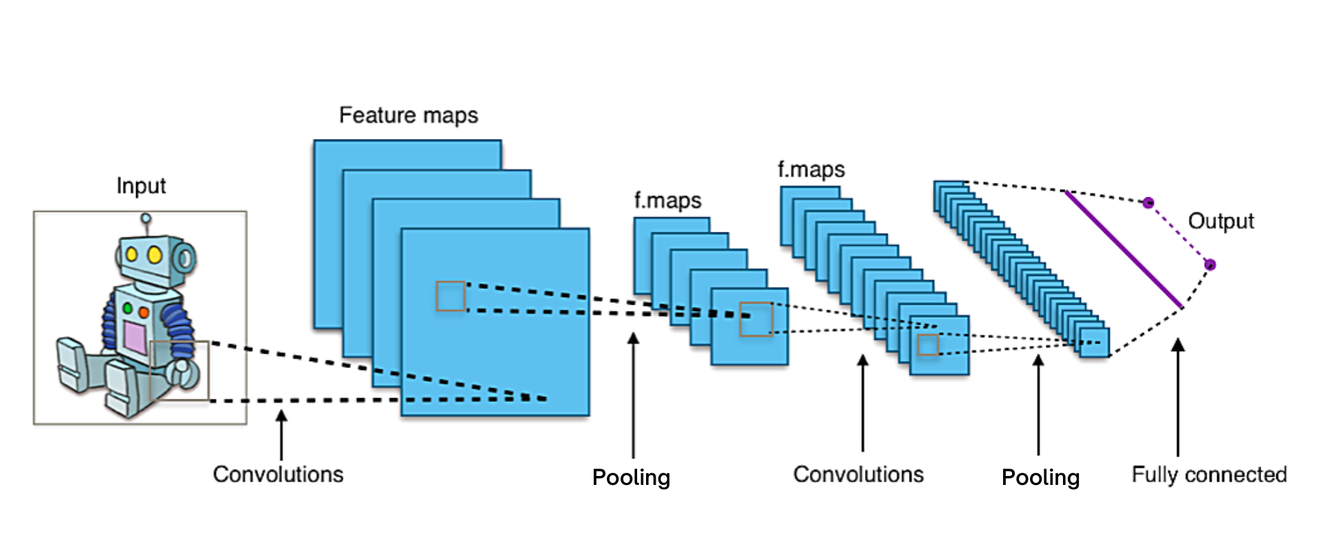
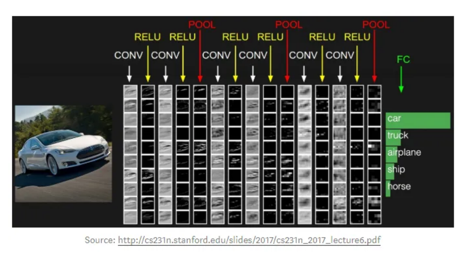
A convolutional network's first layer is the convolutional layer. The fully-connected layer is the last layer, even though convolutional layers, further convolutional layers, or pooling layers, can come after it. The CNN becomes more complicated with each layer, detecting larger areas of the image. Early layers emphasise basic elements like colours and borders. The larger features or shapes of the object are first recognised when the visual data moves through the CNN layers, and eventually the intended object is recognised.

Convolutional Layer

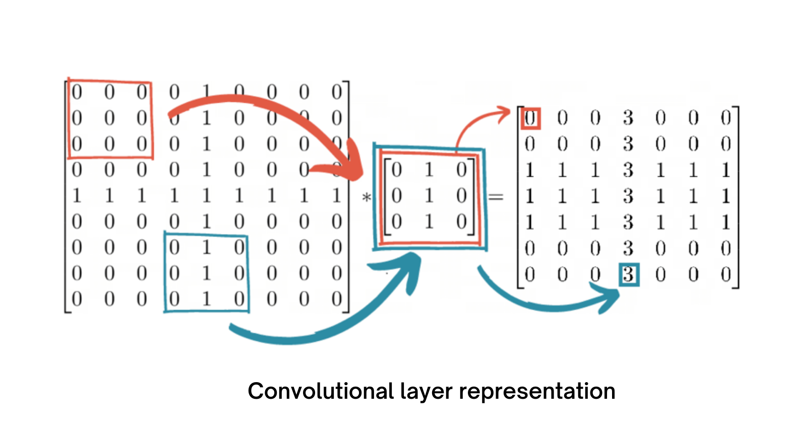
The central component of a CNN is the convolutional layer, which is also where the majority of computation takes place. It needs input data, a filter, and a feature map, among other things. Assume that the input will be a colour image that is composed of a 3D pixel matrix. As a result, the input will have three dimensions—height, width, and depth—that are analogous to RGB in an image. Additionally, we have a feature detector, also referred to as a kernel or filter, which will move through the image's receptive fields and determine whether the feature is there. Convolution describes this process.

A two-dimensional (2-D) array of weights serving as the feature detector represents a portion of the image. The filter size, which also controls the size of the receptive field, is normally a 3x3 matrix, however they can vary in size. Following the application of the filter to a portion of the image, the dot product between the input pixels and the filter is determined. The output array is then fed with this dot product. Once the kernel has swept through the entire image, the filter shifts by a stride and repeats the operation. A feature map, activation map, or convolved feature is the ultimate result of the sequence of dot products from the input and the filter.

A CNN performs a Rectified Linear Unit (ReLU) adjustment on the feature map following each convolution operation, adding nonlinearity to the model.

As was previously mentioned, the first convolution layer may be followed by another convolution layer. When this occurs, the CNN's structure may become hierarchical because the later layers will be able to view the pixels in the earlier layers' receptive fields. Let's use the case of trying to determine whether a bicycle is there in an image as an example. The bicycle can be viewed as a collection of components. It has a frame, handlebars, wheels, pedals, and other parts. A feature hierarchy is created within the CNN by the bicycle's component pieces, each of which represents a lower-level pattern in the neural network and the bicycle as a whole a higher-level pattern.

Pooling Layer

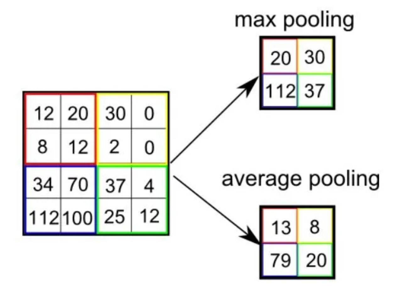
Downsampling, also referred to as pooling layers, carries out dimensionality reduction and lowers the amount of parameters in the input. The pooling operation spreads a filter across the whole input similarly towards the convolutional layer, with the exception that this filter lacks weights. Instead, the kernel populates the output array by applying an aggregation function to the numbers in the receptive field. The two primary forms of pooling are :

1. Max pooling: The filter chooses the pixel with the highest value to send to the output array as it advances across the input. As a side note, this method is applied more frequently than average pooling.

2. Average pooling: The filter calculates the average value inside the receptive field as it passes across the input and sends that value to the output array.

The pooling layer loses a lot of information, but it also offers the CNN a number of advantages. They lessen complexity, increase effectiveness, and lower the risk of overfitting.

Fully-Connected Layer

The full-connected layer is exactly what its name implies. As was already noted, partially connected layers do not have a direct connection between the input image's pixel values and the output layer. In contrast, every node in the output layer of the fully-connected layer is directly connected to a node in the layer above it.

Based on the features that were retrieved from the preceding layers and their various filters, this layer conducts the classification operation. FC layers often utilise a softmax activation function to categorise inputs appropriately, producing a probability ranging from 0 to 1. Convolutional and pooling layers typically use ReLu functions.

Types of convolutional neural networks

In their respective studies from 1980 and 1989 (Backpropagation Applied to Handwritten Zip Code Recognition), Kunihiko Fukushima and Yann LeCun provided the groundwork for research on convolutional neural networks. The more well-known example is when Yann LeCun used backpropagation to train neural networks to recognise patterns in a set of handwritten zip codes. Throughout the 1990s, he and his colleagues would continue their study, culminating in "LeNet-5," which used the same concepts from earlier studies to recognise documents. With the release of new datasets like MNIST and CIFAR-10 and competitions like ImageNet Large Scale Visual Recognition Challenge, a variety of variant CNN architectures have now evolved (ILSVRC).

CNN machine learning models can represent the slightly elevated representation of the input data by applying several convolutional filters, making CNN techniques very common in computer vision tasks. Examples of convolutional neural network applications include object detection and image categorization (using tools like AlexNet, VGG network, ResNet, and MobileNet) (e.g., Fast R-CNN, Mask R-CNN, YOLO, SSD).

1. AlexNet

AlexNet, the first CNN neural network to triumph in the 2012 ImageNet Challenge, has three fully connected layers and five convolutional layers for image categorization. In order to categorise the image with a size of 227227, AlexNet needs 61 million weights and 724 million MACs (multiply-add computation).

2. VGG-16

In order to categorise the image with a size of 224224, the VGG-16 is trained to a deeper structure of 16 layers, comprising of 13 convolutional layers and 3 fully connected layers, using 138 million weights and 15.5G MACs.

3. GoogleNet

The introduction of an inception module made up of various sized filters by GoogleNet aims to increase accuracy while minimising the computation required for DNN inference. As a consequence, GoogleNet outperforms VGG-16 in accuracy performance despite processing an image of the same size with only seven million weights and 1.43G MACs.

4. ResNet

ResNet, a cutting-edge project, uses the "shortcut" structure to achieve accuracy comparable to that of a person and a top-5 error rate under 5%. In order to train a DNN model with a deeper structure, the "shortcut" module is also utilised to address the gradient vanishing issue during training.

LeNet-5 is regarded as the traditional CNN architecture, though.

Convolutional neural networks (CNNs) vs Other neural networks

Regular neural networks' (NNs') main drawback is their inability to scale. A conventional NN might deliver acceptable results for smaller images with fewer colour channels. However, as an image's size and complexity grow, so does the demand for processing power and resources, necessitating a bigger, more expensive NN.

Additionally, overfitting, where the NN tries to learn too many specifics from the training data, becomes an issue over time. Additionally, it can wind up learning the data noise, which has an impact on how well it performs with test data sets. In the end, the NN is unable to recognise the characteristics or patterns in the data set, and consequently, the object itself.

A CNN, on the other hand, employs parameter sharing. Every node in a CNN layer is connected to every other node. As the layers' filters traverse over the image, a CNN also has a corresponding weight; this is referred to as parameter sharing. Because of this, the entire CNN system requires less processing than a NN system.

Convolutional neural networks applications

Computer vision and image recognition activities are powered by convolutional neural networks. Artificial intelligence (AIfield )'s of computer vision enables computers and systems to extract useful information from digital pictures, movies, and other visual inputs and to behave accordingly. It differs from picture recognition jobs in that it can make recommendations. Current examples of typical uses for this computer vision include:

Healthcare

Since the digitalisation of health records and images, the health sector has reaped significant benefits from deep learning capabilities. Image recognition software can help diagnostic imaging specialists and radiologists analyse and evaluate more images in much less time.

Automotive

Research in automated vehicles and self-driving automobiles is being powered by CNN technology.

Social media

Social media sites employ CNNs to recognise individuals in a user's photo and enable the user to tag friends.

Retail

Brands can recommend goods that are likely to appeal to a customer on e-commerce platforms that use visual search.

Facial recognition for law enforcement

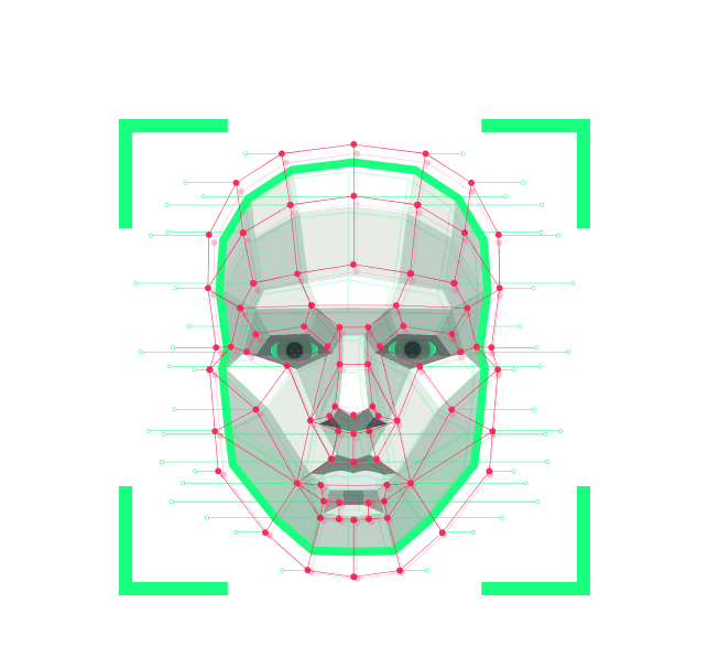
Deep learning algorithms for facial recognition are trained using fresh photos created by generative adversarial networks (GANs).

Audio processing for virtual assistants

Virtual assistants employ CNNs, which learn and recognise user-spoken keywords and process information to direct their actions and communicate with the user.

Advantages of Convolutional Neural Networks

1. Excellent in spotting patterns and characteristics in signals like as photos, movies, and sounds.

2. Resistant to scaling, rotation, and translation invariance.

3. There's no need for manually extracting features with end-to-end training.

4. Can attain excellent accuracy while handling massive amounts of data.

Disadvantages of Convolutional Neural Networks

1. Expensive to train computationally and memory-intensive.

2. Insufficient data or improper regularisation might lead to overfitting.

3. Need a lot of data that has been tagged.

4. Limited interpretability makes it challenging to comprehend what the network has discovered.

FAQs

1. What is deep learning?

Deep learning is a type of machine learning which uses algorithm analysis to automatically learn and enhance functionality. Artificial neural networks are used by the algorithms to learn and enhance their performance by mimicking how people think and acquire knowledge.

2. What is deep learning Good For?

A form of machine learning known as "deep learning" combines algorithm analysis to dynamically learn and improve functionality. The algorithms learn and improve their performance by imitating how individuals think and learn using artificial neural networks.

3. Why is deep learning used?

Large-scale data interpretation and information generation are made quicker and simpler using deep learning. It is employed in a variety of sectors, including automated driving and medical equipment.

4. How does deep learning relate to neural networks?

Deep learning uses and acts on neural networks. The neural networks help to make learning happen by supporting the process.

5. How does AI compare to deep learning?

AI comes in many forms, including machine learning and deep learning. Artificial intelligence is a subset of machine learning, which is a subset of deep learning. Machine learning can automatically adapt with little human intervention thanks to deep learning, which uses artificial neural networks to simulate the learning process in the human brain.

Conclusions

This concludes our discussion of "Convolutional Neural Networks". I sincerely hope that you learned something from it and that it improved your knowledge. You can visit logicmojo to learn more about other topic related to this field.

Good luck and happy learning!