Choose a Language

Experts to solve your doubts in Lectures & Assignments
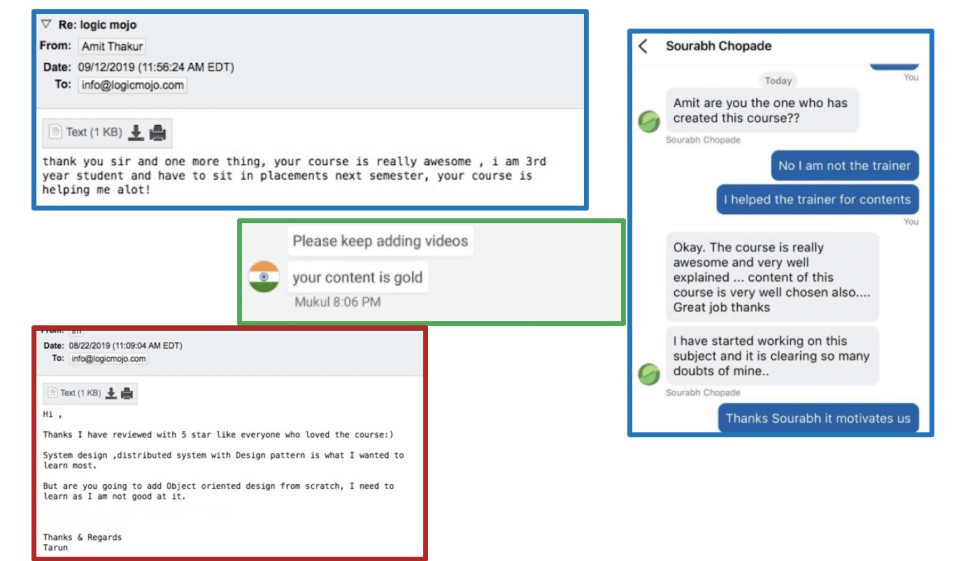
Solve your everyday’s doubts by
By Team of Top tech developers of 10+ exp.


Solve your everyday’s doubts by
By Team of Top tech developers of 10+ exp.


Must recommend for the aspirants who are preparing for Amazon, Google, Microsoft and Top Product Based Company interview


The course curriculum is of best quality along with good coding problems.It's like a quick interview preparation guide


Excellent course for interview preparation, very straight to the point ,in depth coverage of every point. Nice way of explaining solutions to very complex problems in easy way


I would say the best part is the explanation by the instructor, concise and clear. Great quality online content and video lectures, it covers all algorithms and system design problems asked during interviews


Great course! Definitely helped me open some new doors in understanding how algorithms work and implementing solutions for the different exercises
Must recommend for the aspirants who are preparing for Amazon, Google, Microsoft and Top Product Based Company interview
The course curriculum is of best quality along with good coding problems.It's like a quick interview preparation guide
Excellent course for interview preparation, very straight to the point ,in depth coverage of every point. Nice way of explaining solutions to very complex problems in easy way
I would say the best part is the explanation by the instructor, concise and clear. Great quality online content and video lectures, it covers all algorithms and system design problems asked during interviews
Great course! Definitely helped me open some new doors in understanding how algorithms work and implementing solutions for the different exercises


 Experienced Candidate Apply 20% Discount
Life Time Access Course (250+ Lectures)
1+ to 15 years of work exp. in any domain
Online Program
5950/-
 Experienced Candidate Apply 20% Discount
Life Time Access Course (250+ Lectures)
1+ to 15 years of work exp. in any domain
Online Program
5950/-
 Freshers Candidate Apply 20% Discount
Life Time Access Course (240+ Lectures)
Undergraduates, Fresher, 1 Year exp
Online Program
4950/-
 Freshers Candidate Apply 20% Discount
Life Time Access Course (240+ Lectures)
Undergraduates, Fresher, 1 Year exp
Online Program
4950/-
This course will make your interview preparation process very easy. It's not about solving every problem of every topic but it's about practicing similar problems to understand the tricks. Once you know the tricks then any problems can be solved easily.
We have 250+ Lectures of All topics of data structure , Algorithms & System Design. Each topic explains from a very basic to advanced level by using multiple examples. More focus is on Tricks,Techniques and implementation than theory.
We have assignments with every lecture on every topic. After understanding lectures give it a shot to assignments that are based on similar concepts of lectures. Even if you can't able to crack assignments by yourself, we have all assignments in detail discussion with code explanation.
In this course, we teach all techniques of solving algorithms with the help of (Lectures + Assignments) combo.
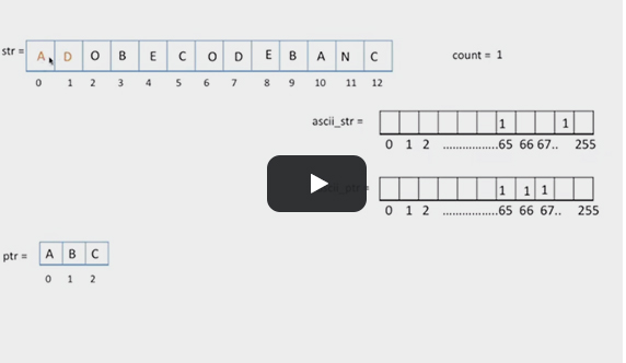
How about Analyzing every code with step by step execution with diagrams and pointers. Yes! You can analyse by yourself every code line by line.
Visual memory is always better for understanding code. This is a new technique of step by step analyzing code with diagrams, blocks, and pointers. Techniques for analyzing code will help you to complete your interview preparation fast. Learning code flow from this technique will always make you ahead of other aspirants. Try Yourself and see how it Works!!
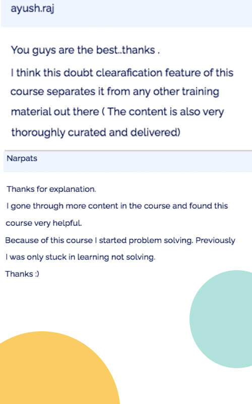
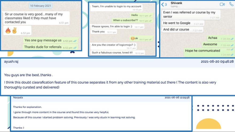
Doubt clearing program by our experts. Every lectures has doubts clearing option where user can ask there doubts related to that lecture. Also, they can include code,voice screen record or screenshot. All queries will answered by our experts.
Main purpose of Interview is to test the candidates coding skills.We provide online editors to practice lectures and assignments in Java/Python Language.

It is also very important to test subscribers progress while preparing for the course. We have online coding tests for specific topics every week in Data Structure & Algorithms. We keep track of your progress during the course preparation program. These Online tests for every topic will brush up coding skills
For every lecture, we provide a complete code solution in your favourite editor in java and python. For assignments you can also practise code in editor
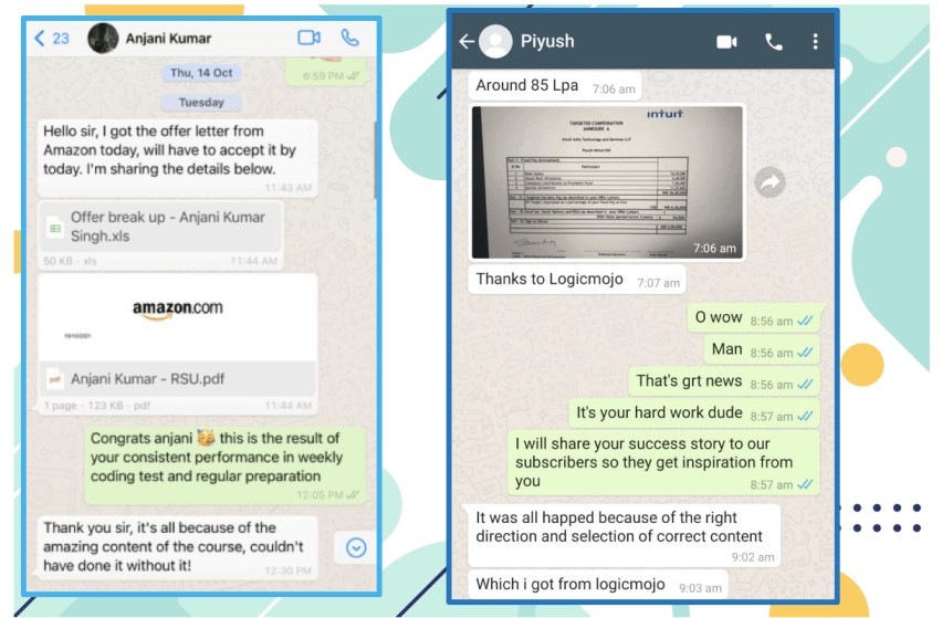
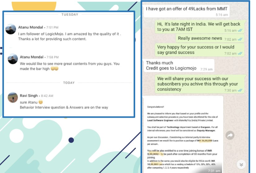
There is a Job referral programs in top product based companies but it has one constraint that you also need to put your efforts and perform in a weekly online coding test.
All the performant subscribers will be eligible for Mock interviews as well as Job referral program.


Most developers struggle with the system design interview, partly because of their lack of experience in developing large-scale systems and partly because of the lack of complete understanding scalable design components This Course is complete guide to master in System Design Interview

Design Facebook's Newsfeed, which would contain posts, photos, videos, and status updates from all the people

Design scalable URL shortening service like TinyURL. This service will provide short aliases for all long URLs

Design a video sharing service like Youtube. This service is accessed by billions,User can upload,search and view the videos

Online distributed Movie ticket booking system where a user can search a movie in a given city and book ticket through payment gateway

Design complex ride sharing service like Uber where system track millions of drivers and customers location

Design an instant messaging service like Whatsapp and Facebook Messenger where a user can send the instant message to other user

Design a social networking service like twitter, where users can post tweet and follow others users

Design a photo-sharing service like Instagram

Design a file hosting service like Dropbox or Google Drive. Millions of users can upload/download documents

An Airline Management System is a managerial software which provide transport services for their passengers

Online shopping system like Amazon where user can place various items in a cart and place an order

Design Object Oriented Design of Chess game which is played between two players and relationship of all classes

Design a System like Cricinfo which provides live tracking of match every ball along with all the players details

Design the data structures for a generic Deck of Cards and Blackjack Game by using objected oriented principal

Design online hotel booking system (Like oyo, agoda) where user can reserve/cancel booking of different types of rooms

Design a discussion forum where members can comments, ask questions or provide answers to the question

Design Multi-Level car parking system using Object Oriented Pricipal

Single Responsibility Open/Closed principle Liskov principal,Interface Segregation Dependency Inversion Principle

Factory method is creational design pattern, this method provides one of the best ways to create an object

Builder Design pattern designed to provide a flexible solution to creating complex in oops programming

Adapter pattern makes two incompatible interfaces compatible without changing their existing code

Decorator pattern is a design pattern that allows behavior to be added to an individual object,dynamically

Observer design pattern has a one-to-many relationship so that when one object changes state, the others are notified and updated automatically

singleton class is a class that can have only one object at a time

Strategy design pattern helps to choose a specific implementation of algorithm or task in run time

Abstract factory pattern provides a way to encapsulate a group of individual factories that have a common theme

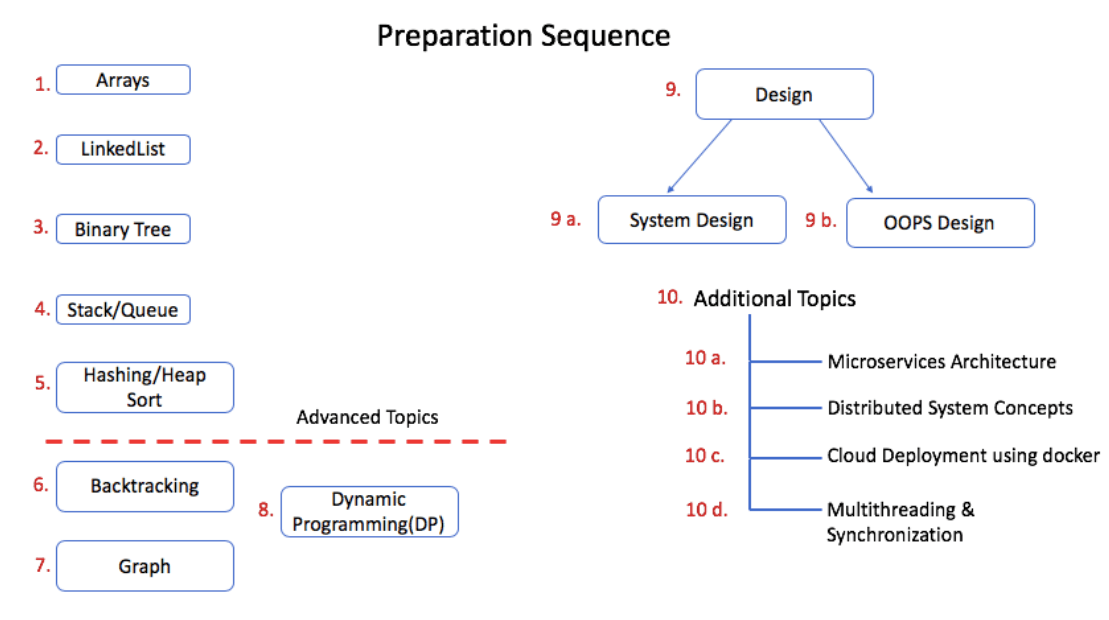
This course is divided into multiple topics. Subscribers can finish topics one after another. The preparation sequence of the course and time to accomplished every topic is already shared in the course brochure

We organized an Online weekly coding test for all subscribers of Logicmojo. Every week we have a coding competition on one specific topic of DSA. Every week subscribers learn and practice topics in a coding competition.

All top performers will be eligible for Mock Interview and Resume Guidelines by experts as well as they are intelligible for Job referral program for FREE
All performers also eligible for our Job referral program through partnered consultancies and software companies for coding interviews
Please note Data structure, Algorithms and Problem Solving only required for cracking top product companies interview across the globe. After selection in any company, you will eventually use their tools, API's and in-built libraries to develop the products.
So,You need to prepare for coding and system design interviews very smartly. Rather than solving thousands of problems from Leetcode and investing 1+ years of time frame. Prepare from the course, all the concepts & problem-solving techniques and finish your preparation in few months.
Once you are shortlisted in your desired organization, then definitely practice from leetcode, participate in CodeChef, Topcoder & Bootcamp coding tests.
As much you practice it will eventually improve your coding skills.
Just Click on "Enroll Now"for registration. During registration you need to provide a mobile Number then you click on the "Generate Coupon Code" Button and the coupon code will come to the subscriber mobile
Subscribe apply that discount coupon and price of the course will reduce further
2 Months to 2.5 Months
If you just spend 2 hours every day in this course then in 2 to 2.5 months of time frame your preparation of coding and system design interview will be done.
You dont even need to refer to any other resources just finish this course and you are good to go for Top Tech Interviews
Yes!!
Subscribers can access all lectures for lifetime. They can access all lecture any time and any place. Also, subscribers will also get all updates that will come in the future.
Just Click on "Enroll Now" and Subscribe for the course
Users can participate in Online Weekly Code forever but Doubt clearing session will be available for 5 month period
We want candidates should also put their effort into completing the course and participate in the Weekly online coding test. All the performant subscribers in the coding test will be eligible for Mock interviews as well as Job referral program
The weekly coding test is on hackerrank platform with 2 problems and 90 min of time frame.
There is no limit on the number of weekly coding test subscribers who want to attend. Subscribers can attend these weekly coding tests at any time. So, It's advisable they should start participating in the weekly coding test when they feel confident on a particular topic.
Yes, every problem in this course is explained with code and examples. Our main intension is to make the programming skills of our candidates strong. So line by line code explains while solving any problems
We don't put any constraint of the batch system in our course, as soon as aspirant subscribe for the course complete course content will be available
Batch System always restricts aspirants for accessing the complete course. If a student has an interview after a few weeks and he/she want to prepare for advanced topics, then the batch system will not allow accessing the course content
Yes, you can access the complete course in Mobile or Tablet

PHONE: +91 80889-75867
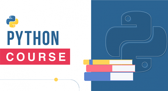
Logicmojo is an Online coding interview preparation course for Cracking the Coding Interview in Amazon, Microsoft, Google & all FAANG companies. All Tech Giant Companies have 3-4 rounds to test candidate's coding skills. In this course we teach the aspirants from very basic to complete advance for cracking the coding interview in product companies, also we support Python & Java languages. Although Data Structure, Algorithms are considered to be independent of languages. Using any language you can implement your code.
Every Language has different features & properties but globally mostly developers prefer Java, Python, or C++ for problem-solving. So you can prepare and Cracking the coding interview by using Python/java.
This is an end-to-end Coding Interview preparation course where along with Data structure, Algorithms & problem Solving, we cover System Design interviews preparation & Distributed Components also
Just watching lectures is not enough you need to practice every problem in our supported editor and try to pass all test cases. If you get stuck while solving any problem please refer code explanation for help or ask any doubts with our team of experts. Cracking the coding interview in Amazon, Google or any FAANG company requires lots of practice.
We have two courses one for freshers and the other for experienced candidates. It has data structure interview questions for experienced as well as data structure interview questions for freshers. These data structure interview questions for freshers as well as experienced mostly repeated problems in product companies interviews. No need to break your head with a huge set of contents Online. You can master the coding interview preparation for data structures + algorithms problems within 2-3 months. We explain all data structure interview questions in java & Python languages.
We start from an array and then step by step move to advanced topics like Graph & DP. Gradually, you become a master in the coding interview by learning data structures + algorithms problem-solving techniques. Usually, DSA is independent of languages but in this course, we teach code explanation of all data structure interview questions in java and Python
Yes, it is mandatory. If you have more than 1 year of experience in the industry. System design interview questions must be there in at least one round of interviews. System design interview preparation requires a deep understanding of distributed components as well as oops concepts. In this course, we cover end to end all aspects of System Design problems from basic to complete advanced with 40+ system design interview questions collection asked in FAANG companies
 Cracking The Coding &
  Cracking The Coding &
  Cracking The Coding &
  Cracking The Coding &