Unlock the complete
Logicmojo experience for FREE
Sign Up Using
1 Million +
Strong Tech Community
500 +
Questions to Practice
100 +
Expert Interview Guides
Sign Up Using
Strong Tech Community
Questions to Practice
Expert Interview Guides

In the field of statistics and data analysis, the correlation coefficient plays a vital role in measuring the relationship between two variables. It provides insights into how changes in one variable correspond to changes in another. In this article, we will explore the concept of correlation coefficient, its types, interpretation, calculation methods, and its various applications.
Sometimes, life is as clear as mud. Ever tried to explain the correlation between your morning coffee and productivity level, or the relationship between rainfall and traffic congestion? Tricky, isn't it? But fret not, because the "correlation coefficient" rides to the rescue. As mysterious as it sounds, it's your statistical superhero, here to save the day.
 Learn More️
A correlation coefficient is a numerical metric in statistics that represents the degree and direction of a linear relationship between two variables. It quantifies the degree to which changes in one variable are related to changes in the other. The correlation coefficient is represented by the symbol "r" and ranges from -1 to 1. A positive value of "r" shows a positive association, which means that as one variable increases, so does the other. A negative r value shows a negative association in which one variable tends to increase while the other variable tends to decline.
The correlation coefficient's magnitude indicates how strong the association is. A strong association is indicated if the absolute value of r is close to 1, whereas a weak relationship is suggested by values closer to 0. Noting that correlation does not indicate causation is crucial. It's not always the case that changes in one variable result in changes in the other, even when two variables are connected. Only the statistical relationship between variables is measured by correlation.
Data science, business analytics, and other buzzwords in the sector are frequently used interchangeably. In reality, these phrases refer to particular subsets of data that are crucial to the various phases of data utilization. The correct handling of data in the digital age involves a lot of moving parts, therefore data analytics should be approached as a whole program rather than as a collection of specialized tools.
The interpretation of correlation coefficients is crucial for understanding the relationship between two variables. By examining the values of correlation coefficients, we can gain insights into the nature and strength of the association between the variables.
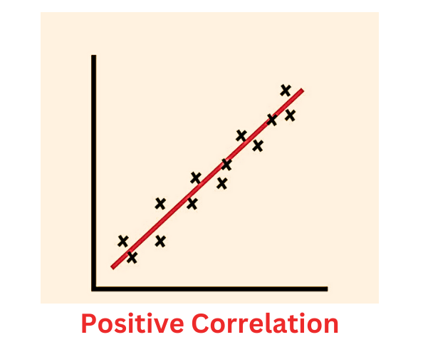
When we encounter a positive correlation coefficient, it indicates a direct relationship between the variables. In simpler terms, as one variable increases, the other variable tends to increase as well. For example, suppose we are examining the correlation between study hours and academic performance. A positive correlation coefficient suggests that students who spend more time studying generally achieve higher grades.
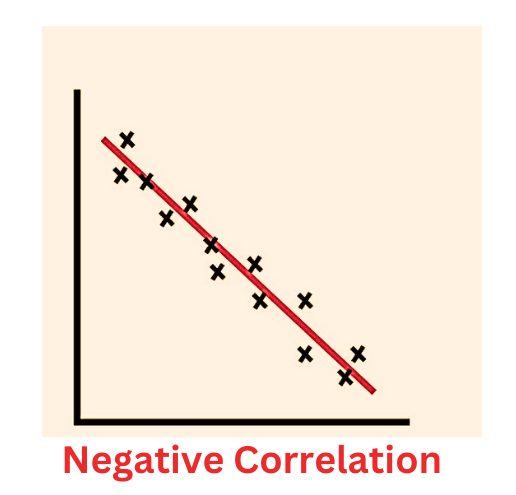
On the flip side, an antagonistic correlation coefficient signifies an opposing relationship. In this scenario, as one factor escalates, the other factor tends to diminish. Employing the identical illustration, if we discover an antagonistic correlation between the amount of time dedicated to studying and the tally of errors committed on a examination, it implies that as the study hours increase, the number of errors decreases.
To further grasp the intensity of the association, we scrutinize the magnitude of the correlation coefficient. The closer the correlation coefficient approaches +1 or -1, the more robust the connection between the variables becomes. For instance, a correlation coefficient of +0.9 or -0.9 indicates an exceedingly potent correlation, signifying that the variables are profoundly interconnected. Conversely, a correlation coefficient in proximity to 0 indicates a feeble or absent linear relationship. In this instance, alterations in one variable do not consistently correspond to modifications in the other variable.
While correlation coefficients provide valuable insights into the statistical association between variables, it's important to remember that correlation does not imply causation. Even if a strong correlation exists, it does not establish a cause-and-effect relationship between the variables. There may be other underlying factors or coincidences influencing the observed correlation.
For example, a positive correlation between ice cream sales and sunglasses purchases during the summer does not mean that buying sunglasses causes people to buy more ice cream.
By considering these factors, we can interpret correlation coefficients more accurately and avoid drawing unwarranted conclusions. It is essential to conduct further research and analysis to understand the underlying mechanisms and potential confounding variables that may influence the observed relationship.
Let us delve into a couple of instances to exemplify the notion of correlation coefficients:
Visualize our curiosity regarding the connection between an individual's Height and Weight. To explore this matter, we amass data from a cohort of individuals, documenting their heights and corresponding Weight. By computing the correlation coefficient, we can evaluate the affiliation between these variables. If the resultant correlation coefficient approximates +1, it signifies a robust positive correlation. Within this context, it implies that individuals with greater height tend to possess higher Weight. Nonetheless, it is crucial to acknowledge that correlation does not infer causation. Other factors, such as genetics, lifestyle, and diet, can also impact an individual's Weight.
Imagine a scenario where we yearn to investigate the interplay between temperature and Ice Cream vending. To scrutinize this interrelationship, we gather data concerning temperature and the corresponding everyday Ice Cream sales. Through the computation of the correlation coefficient, we can ascertain the degree of association between these variables. If we detect a positive correlation coefficient, it suggests that as temperature escalates, Ice Cream sales also demonstrate an incline. This positive correlation indicates that warmer weather stimulates people to indulge in frozen delights. Nevertheless, it is crucial to recognize that correlation unaided cannot establish a causal bond. Other factors, such as marketing endeavors or seasonal patterns, might also exert influence on Ice Cream sales.
These instances serve as manifestations of how correlation coefficients can proffer insights into the connection between variables. They enable us to quantify the potency and direction of the affiliation, empowering us to make knowledgeable interpretations and predictions. Nevertheless, it is imperative to conduct further analysis and contemplate supplementary factors to attain a comprehensive comprehension of the underlying dynamics.
Learn From Basic to Advanced Data Structures, Algorithms & Problem-Solving techniques in Java

1:1 Mentorship
4 Months Classes
LIVE Classes Weekend
Projects included

Learn From Basic to Advanced DSA, Problem Solving, Scalable System Design (HLD + LLD),Design Patten in Java
1:1 Mentorship
7 Months Classes
LIVE Classes Weekend
Projects included
Now we will look into more questions related to Correlation Coefficient to know about differents types and its applications and many more things.
Distinct forms of correlation coefficients are frequently utilized to capture distinct aspects of the association when studying the link between variables. Let's delve deeper into each of these correlation indices:
The most commonly used correlation metric is Pearson's correlation coefficient, abbreviated "r." The linear link between two continuous variables is quantified. The normal distribution of the variables is assumed by this coefficient. R has a value between -1 and +1, with 0 denoting a linear connection. If the value is positive, there is a positive correlation between the two variables, which means that if one variable rises, the other tends to rise as well. Conversely, a negative value suggests a negative correlation, implying that as one variable increases, the other tends to decrease.
Spearman's rank correlation coefficient, denoted as "ρ" (rho), is a non-parametric measure of correlation. It assesses the monotonic relationship between variables, meaning it captures whether the variables tend to change together in a consistent manner, without assuming a specific form of the relationship. Spearman's correlation coefficient is suitable for variables measured on an ordinal scale or when the relationship is not strictly linear. It is calculated by converting the original values of the variables into ranks and then applying Pearson's correlation coefficient to the ranks. Like Pearson's correlation coefficient, the value of Spearman's ρ ranges from -1 to +1, with 0 indicating no monotonic relationship.
Kendall's tau, denoted as "τ" (tau), is another non-parametric correlation coefficient used to measure the ordinal association between variables. It assesses the strength and direction of the relationship without assuming linearity. Kendall's tau is particularly useful when dealing with ranked or categorical data. It quantifies the number of concordant and discordant pairs of observations and calculates the probability of observing such pairs. Like the other correlation coefficients, Kendall's tau ranges from -1 to +1, where 0 indicates no association.
These different types of correlation coefficients provide flexibility in capturing various types of relationships. Pearson's correlation coefficient is suitable for assessing linear associations between continuous variables, while Spearman's rank correlation coefficient and Kendall's tau are more appropriate for capturing monotonic and ordinal relationships, respectively. Choosing the right correlation coefficient depends on the nature of the variables and the type of relationship under investigation.
Although data analytics techniques vary from application to application, they all fall into one or more of the following categories:
The Strength of a correlation coefficient, such as Pearson's correlation coefficient (r), offers valuable insights into the intensity of the association between two variables. Evaluating the extent of the correlation coefficient allows us to gauge the strength of the relationship.
When the correlation coefficient approaches -1 or +1, it signifies a robust correlation between the variables. A coefficient of -1 represents a perfect negative correlation, where one variable consistently decreases as the other variable increases in a predictable manner. Conversely, a coefficient of +1 represents a perfect positive correlation, where both variables consistently increase together in a predictable manner. In these instances, the relationship between the variables is highly pronounced and dependable.
For example, let's consider a study investigating the connection between age and reaction time. If the computed correlation coefficient approaches -1, it suggests a strong negative correlation. This indicates that as age advances, reaction time tends to decrease consistently, reflecting a robust negative association. Conversely, if the correlation coefficient approaches +1, it implies a strong positive correlation. This indicates that as age increases, reaction time also increases consistently, demonstrating a pronounced positive relationship.
Conversely, when the correlation coefficient approximates 0, it indicates a weak or negligible correlation between the variables. This implies that changes in one variable do not consistently correspond to changes in the other variable. The relationship is less prominent and predictable.
For instance, let's contemplate a study exploring the link between shoe size and intelligence. If the computed correlation coefficient approximates 0, it suggests a weak or negligible correlation between these variables. This signifies that shoe size is not a reliable predictor of intelligence since there is no consistent pattern between the two.
It is important to note that a correlation coefficient of 0 does not necessarily indicate the absence of any relationship between the variables. There might still be other types of relationships, such as nonlinear relationships or relationships that are not captured by Pearson's correlation coefficient. Therefore, it is vital to consider additional analyses and contextual information to gain a comprehensive understanding of the relationship between the variables.
To summarize, the strength of a correlation coefficient is determined by its proximity to -1 or +1. Values closer to these extremes indicate a strong correlation, while values closer to 0 suggest a weak or negligible correlation between the variables.
Find the standard deviation of each variable and the covariance between them before calculating the Pearson correlation. The correlation coefficient is calculated by dividing the covariance by the sum of the standard deviations of the two variables.
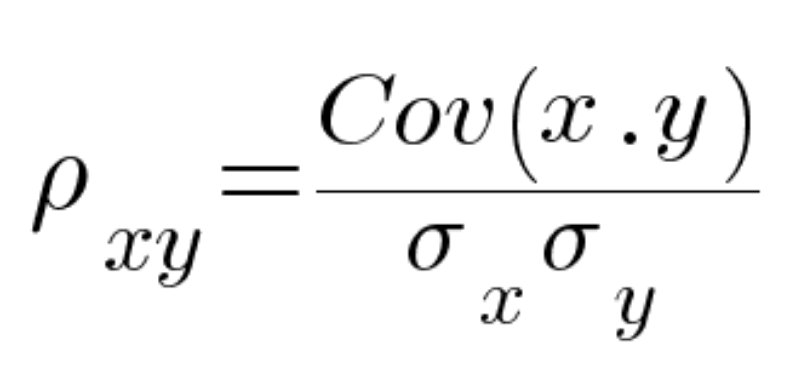
Where,
ρxy = The Pearson product-moment correlation coefficient
Cov(x,y) = covariance of the variables x and y
σx = standard deviation of x
σy = standard deviation of y
The standard deviation is a measurement of how far apart the data are from the mean. The correlation coefficient quantifies the strength of the association between the two variables on a normalized scale from -1 to 1, whereas covariance indicates whether the two variables tend to move in the same direction.
The strength and direction of the linear link between two variables are measured by the correlation coefficient. The Pearson correlation coefficient, abbreviated "r," is the most often used correlation coefficient. This mathematical equation is used to compute it:
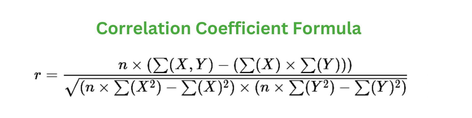
X and Y represent the values of the two variables.
X̄ and Ȳ represent the means (averages) of X and Y, respectively.
Σ denotes summation, which means adding up the values.
To calculate r, the equation involves three main steps:
Calculate the difference between each value of X and the mean of X (X - X̄), and the difference between each value of Y and the mean of Y (Y - Ȳ).
Multiply these differences for each data point ( (X - X̄) * (Y - Ȳ) ) and sum up these products.
Divide the sum of the products by the square root of the product of the sum of the squared differences for X ( Σ((X - X̄)^2) ) and the sum of the squared differences for Y ( Σ((Y - Ȳ)^2) ).
By calculating this equation, we obtain the correlation coefficient (r), which will be a value between -1 and +1. The sign (+/-) of r indicates the direction of the relationship, while the magnitude represents the strength of the relationship. A positive value of r indicates a positive correlation, a negative value indicates a negative correlation, and a value close to 0 suggests a weak or no linear relationship between the variables.
It's important to note that this equation specifically calculates Pearson's correlation coefficient (r) for two continuous variables assuming a linear relationship. Different equations, such as Spearman's rank correlation coefficient and Kendall's tau, are used for variables measured on an ordinal scale or when the relationship is not strictly linear.
To find the correlation coefficient between two variables, you can follow these steps:
Step 1: Collect Data
Collect a set of data pairs that represent the values of the two variables you want to analyze. Ensure that you have a sufficient number of data points to obtain a reliable correlation coefficient.
Step 2: Calculate the Means
Calculate the mean (average) of both variables. Let's denote the mean of variable X as X̄ and the mean of variable Y as Ȳ.
Step 3: Calculate the Differences
For each data point, calculate the difference between the value of X and its mean (X - X̄), as well as the difference between the value of Y and its mean (Y - Ȳ).
Step 4: Calculate the Products
Multiply the differences obtained in Step 3 for each data point. That is, multiply (X - X̄) with (Y - Ȳ) for each data pair
.Step 5: Sum the Products
Sum up all the products calculated in Step 4.
Step 6: Calculate the Sum of Squared Differences
Calculate the sum of the squared differences for X (Σ((X - X̄)^2)) and the sum of the squared differences for Y (Σ((Y - Ȳ)^2)).
Step 7: Calculate the Correlation Coefficient
Divide the sum of the products from Step 5 by the square root of the product of the sum of squared differences for X and the sum of squared differences for Y.
This can be expressed as:
r = (sum of products) / sqrt((sum of squared differences for X) * (sum of squared differences for Y))
The resulting value, denoted as "r," represents the correlation coefficient between the two variables. The correlation coefficient will range from -1 to +1, where -1 indicates a perfect negative correlation, +1 represents a perfect positive correlation, and 0 suggests no linear correlation.
It's important to note that this calculation specifically applies to Pearson's correlation coefficient (r) for two continuous variables assuming a linear relationship. Different calculations, such as using ranks, may be required for Spearman's rank correlation coefficient or Kendall's tau when dealing with other types of variables or non-linear relationships.
Statistics almost always employs correlation. The link between two or more variables is illustrated by correction. The correlation coefficient, which is a number, is used to express it. Most correlations go into one of two categories:
Karl Pearson's correlation coefficient, also known as Pearson's correlation coefficient or simply Pearson's r, relies on certain assumptions when calculating and interpreting the correlation between two variables. These assumptions are important to ensure the validity and meaningfulness of the correlation coefficient:
1. Linearity: Pearson's correlation coefficient assumes a linear relationship between the two variables being analyzed. It measures the strength and direction of the linear association. If the relationship between the variables is not linear, Pearson's correlation coefficient may not accurately capture the underlying association.
2. Normality: The variables involved in calculating Pearson's correlation coefficient should follow a normal distribution. This assumption ensures that the data points are symmetrically distributed around the mean, allowing for more reliable interpretations of the correlation. If the variables are not normally distributed, alternative correlation measures like Spearman's rank correlation coefficient or Kendall's tau may be more appropriate.
3. Homoscedasticity: Homoscedasticity refers to the assumption that the variability of the data points is consistent across all levels of the variables being studied. In other words, the spread or dispersion of the data points should be relatively constant throughout the range of values. Violation of this assumption, known as heteroscedasticity, can affect the accuracy and interpretability of Pearson's correlation coefficient.
4. Independence: The data points used to calculate Pearson's correlation coefficient should be independent of each other. Independence means that the values of one variable are not systematically related to the values of the other variable in a way that would bias the correlation estimation. If there is dependence or autocorrelation between the data points, it can distort the correlation coefficient and lead to inaccurate interpretations.
5. Absence of outliers: Pearson's correlation coefficient is sensitive to extreme values, known as outliers. Outliers can disproportionately influence the correlation estimate and distort the interpretation. Therefore, it is important to identify and handle outliers appropriately before calculating the correlation coefficient.
It is crucial to be aware of these assumptions and assess whether they hold in the specific dataset being analyzed. Violations of these assumptions may require alternative correlation measures or further statistical techniques to ensure accurate analysis and interpretation.
Correlation coefficients, like Pearson's correlation coefficient (r), possess several pivotal characteristics that render them valuable tools for analyzing variable relationships. Here are some key properties of correlation coefficients:
1. Range and Limits: Correlation coefficients span from -1 to +1. A value of -1 signifies a perfect negative correlation, +1 indicates a perfect positive correlation, and 0 denotes no linear correlation. These boundaries offer a clear framework for gauging the strength and direction of the relationship.
2. Symmetry: Correlation coefficients exhibit symmetry, meaning that the correlation between variable X and variable Y is identical to the correlation between variable Y and variable X. Consequently, the variables' order does not impact the correlation coefficient's magnitude or interpretation.
3. Unit-Free: Correlation coefficients are independent of measurement units, making them insensitive to specific units used for variables. The correlation remains unchanged regardless of whether the variables are measured in inches or centimeters, pounds or kilograms, and so on. This property facilitates meaningful comparisons between variables measured in different units.
4. Standardization: Correlation coefficients standardize the variable relationship. By ranging between -1 and +1, they offer a standardized measure of the linear association's strength and direction. This standardization enables comparisons across diverse datasets and variables.
5. Scale Independence: Correlation coefficients remain unaffected by linear transformations of the variables, such as multiplication or division by a constant, or addition or subtraction of a constant value. This property ensures that the correlation coefficient remains consistent even if the variables are rescaled.
6. Sensitivity to Outliers: Correlation coefficients display sensitivity to outliers, which are extreme values deviating significantly from the general data pattern. Outliers can impact the correlation coefficient by exerting disproportionate influence on the calculation. Proper assessment and treatment of outliers are crucial for accurate correlation analysis.
7. Incomplete Measure: Correlation coefficients solely capture the linear relationship between variables. They do not encompass other forms of relationships, including nonlinear associations or interactions. To obtain a comprehensive understanding of variable relationships, it is essential to consider additional analytical techniques and contextual information.
Understanding these properties empowers researchers and analysts to effectively utilize correlation coefficients for assessing and interpreting variable relationships. However, it is vital to remember that correlation does not imply causation, and additional factors may influence observed associations.
Spearman's rank correlation coefficient, often referred to as Spearman's rho (ρ), is a statistical measure used to assess the strength and direction of the monotonic relationship between two variables. It is a non-parametric measure, meaning it does not assume any specific distribution for the variables.
The steps to calculate Spearman's rank correlation coefficient are as follows:
1: Rank the Data
Rank the values of each variable separately, from the smallest to the largest, assigning them ranks accordingly. If there are ties (i.e., multiple data points with the same value), assign them the average rank.
Step 2: Calculate the Differences
Subtract the rank of each data point in one variable from the rank of the corresponding data point in the other variable. These differences represent the pairwise deviations between the ranks.
Step 3: Calculate the Squared Differences
Square each of the differences obtained in Step 2.
Step 4: Calculate Spearman's Rank Correlation Coefficient
Compute the sum of the squared differences obtained in Step 3. Then, use the following formula to calculate Spearman's rank correlation coefficient:
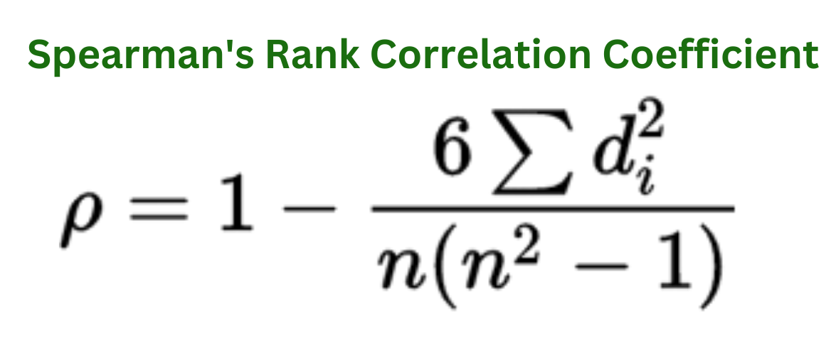
or
ρ = 1 - [(6 * sum of squared differences) / (n * (n^2 - 1))]
In this formula, "n" represents the number of data points in the dataset.
The resulting value of Spearman's rho ranges between -1 and +1. A coefficient of -1 indicates a perfect decreasing monotonic relationship, where higher ranks in one variable correspond to lower ranks in the other variable. A coefficient of +1 signifies a perfect increasing monotonic relationship, where higher ranks in one variable correspond to higher ranks in the other variable. A coefficient close to 0 suggests no monotonic relationship between the variables.
Spearman's rank correlation coefficient is useful when analyzing variables that may not have a linear relationship or when the data violate the assumptions of other correlation measures, such as Pearson's correlation coefficient. It captures the overall monotonic trend between the variables, but it does not provide information about the specific form or shape of the relationship.
It's important to note that Spearman's rank correlation coefficient assesses the strength and direction of the monotonic relationship between variables, but it does not imply causation. Additional analysis and interpretation are necessary to understand the underlying mechanisms and potential confounding factors influencing the observed relationship.
Cramer's V correlation coefficient stands as a statistical measure employed to evaluate the strength and association between two categorical variables. It serves as an extension of the phi coefficient (φ) and finds particular utility when both variables possess more than two categories.
To compute Cramer's V, the subsequent steps are conventionally followed:
Step 1: Construct a Contingency Table
Formulate a contingency table that displays the frequencies or counts of joint occurrences between the two categorical variables. This table comprises rows representing the categories of one variable and columns representing the categories of the other variable.
Step 2: Calculate the Chi-Square Statistic
Determine the chi-square (χ²) statistic based on the contingency table. This statistic assesses the association between the variables, revealing whether a significant relationship exists. However, it does not provide a measure of the association's strength or magnitude.
Step 3: Ascertain the Minimum Dimension of the Contingency Table
To compute Cramer's V, it is imperative to ascertain the minimum dimension of the contingency table. The minimum dimension is obtained by subtracting 1 from the smaller of the two dimensions (rows or columns) in the contingency table.
Step 4: Compute Cramer's V
Finally, calculate Cramer's V correlation coefficient using the following formula:
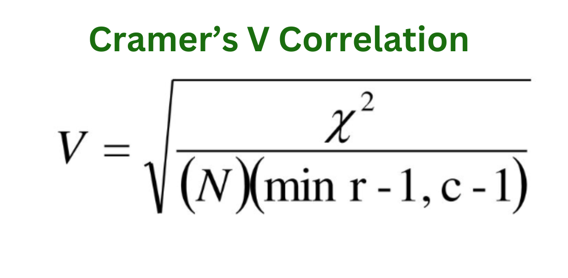
In this formula, χ² denotes the chi-square statistic, n represents the total number of observations or data points, and min_dimension signifies the minimum dimension of the contingency table.
The resulting value of Cramer's V ranges from 0 to 1. A value of 0 indicates no association between the variables, while a value of 1 signifies a perfect association. Intermediate values between 0 and 1 denote varying degrees of association, with higher values indicating stronger associations.
Cramer's V proves especially advantageous when comparing the strength of associations between variables with differing numbers of categories. It furnishes a standardized measure facilitating comparisons across distinct contingency tables.
| Cramer’s V | |
|---|---|
| .25 or higher | Very strong relationship |
| .15 to .25 | Strong relationship |
| .11 to .15 | Moderate relationship |
| .06 to .10 | weak relationship |
| .01 to .05 | No or negligible relationship |
It is important to acknowledge that Cramer's V is designed explicitly for categorical variables and quantifies association rather than causation. Interpretation should be exercised cautiously, taking into account the context and potential confounding factors.
In summary, Cramer's V constitutes a valuable tool for analyzing and quantifying the strength of associations between categorical variables, granting insights into the relationships and patterns within the data.
The notion of correlation can be traced back to the early 19th century, but it was in the late 19th and early 20th centuries that Karl Pearson, an English mathematician and statistician, made notable contributions by introducing the correlation coefficient as a measure of the relationship between two variables.
Pearson's interest in correlation was inspired by the work of Sir Francis Galton, a cousin of Charles Darwin, who examined the connection between heredity and various physical characteristics. Galton initially introduced correlation as a means to describe the relationship between different traits observed among family members, such as height and weight.
Building upon Galton's ideas, Pearson refined and formalized the concept of correlation by developing a calculation method for the correlation coefficient. In his influential paper published in 1895, Pearson introduced what is now known as Pearson's correlation coefficient. This coefficient quantifies the linear relationship between two continuous variables.
Pearson's correlation coefficient originated from the concept of covariance, which measures the variability shared by two variables. Pearson realized that dividing the covariance by the product of the variables' standard deviations would normalize the measure and provide a standardized approach to assess the strength and direction of the linear relationship. This normalization led to the birth of the correlation coefficient, symbolized as "r."
Pearson's work on the correlation coefficient and its statistical properties established it as a fundamental tool in the fields of statistics and data analysis. His contributions laid the groundwork for comprehending and measuring the relationships between variables.
As time passed, other statisticians and researchers developed additional correlation measures, such as Spearman's rank correlation coefficient and Kendall's tau, to accommodate different types of data and relationships. These measures expanded the concept of correlation beyond linear associations, enabling the analysis of monotonic and ordinal relationships.
In contemporary times, correlation coefficients find wide application across various disciplines, including the social sciences, economics, biology, psychology, and more. They furnish valuable insights into the relationships between variables, equipping researchers, analysts, and decision-makers with the means to comprehend and interpret patterns and dependencies within their data.
Karl Pearson's introduction and advancement of the correlation coefficient marked a significant milestone in the realm of statistics, contributing to our understanding of how variables interrelate and exerting influence on diverse areas of research and practical application.
Different correlation coefficients can be visualized using scatter plots, which are graphical representations of the relationship between two variables. Let's explore the graphs for different correlation coefficients:
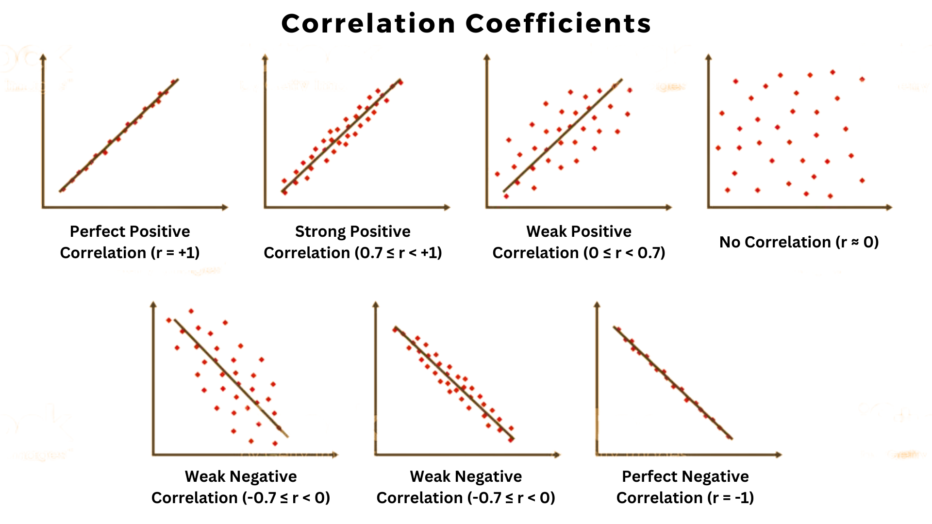
1. Perfect Positive Correlation (r = +1):
In a scatter plot representing a perfect positive correlation, the data points lie on a straight line with a positive slope. As one variable increases, the other variable also increases in a perfectly linear manner. The line connecting the data points starts from the bottom left and goes to the top right of the plot.
2. Strong Positive Correlation (0.7 ≤ r < +1):
For a strong positive correlation, the data points cluster around a rising trend line, indicating a positive relationship. The points have a tendency to be closer to the trend line, although there might be some scattered points. As one variable increases, the other variable generally increases, but not necessarily in a perfectly linear manner.
3. Weak Positive Correlation (0 ≤ r < 0.7):
In a scatter plot representing a weak positive correlation, the data points are more scattered, and the trend line shows a slight positive slope. While there is a general tendency for one variable to increase as the other variable increases, there is also a considerable amount of variation among the data points.
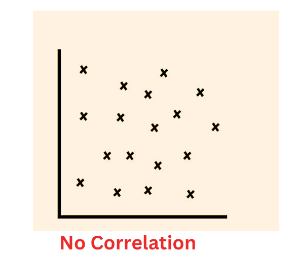
4. No Correlation (r ≈ 0):
In a scatter plot representing no correlation, the data points are scattered randomly without any discernible pattern. The trend line is horizontal, indicating that there is no clear relationship between the variables. Changes in one variable do not correspond to changes in the other variable.
5. Weak Negative Correlation (-0.7 ≤ r < 0):
For a weak negative correlation, the data points tend to scatter around a falling trend line. As one variable increases, the other variable generally decreases, but there is a significant amount of variability among the data points.
6. Strong Negative Correlation (r = -1):
In a scatter plot representing a strong negative correlation, the data points align along a straight line with a negative slope. As one variable increases, the other variable decreases in a perfectly linear manner. The line connecting the data points starts from the top left and goes to the bottom right of the plot.
These graphs visually represent the different correlation coefficients and the corresponding relationships between variables. They provide a clear understanding of how changes in one variable are associated with changes in another variable, depending on the strength and direction of the correlation.
The hypothesis test for correlation coefficients exists. This test, like all hypothesis tests, examines two statements about the population from which the sample was selected that are mutually exclusive. The two hypotheses for Pearson correlations are as follows:
• The two variables don't have a linear connection, which is null. ρ = 0.
• Alternative hypothesis: The two variables have a linear connection. ρ ≠ 0.
Zero correlation coefficients denote the absence of any linear relationship. The sample contains enough data to reject the null hypothesis and draw the conclusion that the Pearson correlation coefficient does not equal zero if your p-value is less than your significance level. In other words, the sample results are consistent with the population-level existence of the link.
An effective correlation is what? What level of correlation coefficients are ideal? These queries are frequently posed. I've come across a number of classification techniques that try to categorize correlations as strong, medium, and weak.
There is only one right response, though. The intensity of the association should be appropriately reflected by a Pearson correlation coefficient. Check out the 0.694 connection between the statistics for height and weight. Although there isn't a lot of association, our data are appropriately represented by it. The ideal case for employing a statistic to describe a whole dataset is an accurate depiction.
Any relationship's strength inevitably depends on the particular pair of variables. Compared to other subject areas, certain research questions require weaker links. Consider how challenging it is to forecast people. Studies that examine human behavior-related relationships typically exhibit correlation coefficients that are weaker than +/- 0.6.
However, you might anticipate correlations approaching +1 or -1 if you examine two variables in a physical process and have extremely accurate observations. No one size fits all ideal answer exists for the strength of a partnership. Depending on your field of study, the appropriate correlation coefficient values will vary.
Understanding the distinction between correlation and causation is crucial in data analysis and interpretation. While correlation measures the statistical relationship between variables, causation refers to the cause-and-effect relationship between variables. It is essential to recognize that correlation does not necessarily imply causation. Let's explore this concept in more detail:
Correlation examines the association or relationship between variables. It measures how changes in one variable relate to changes in another variable. Correlation coefficients, such as Pearson's correlation coefficient, quantify the strength and direction of this statistical association.
A positive correlation indicates that as one variable increases, the other tends to increase as well. A negative correlation suggests that as one variable increases, the other tends to decrease. A correlation coefficient close to zero indicates a weak or no linear relationship between the variables.
Causation, on the other hand, goes beyond the statistical relationship and implies a cause-and-effect connection between variables. It suggests that changes in one variable directly lead to changes in the other variable. Causal relationships involve a mechanism or an underlying reason for the observed effect. Establishing causation requires more rigorous investigation and evidence beyond the observed correlation.
There are several reasons why correlation does not automatically imply causation:
1. Third Variable: Correlation between two variables could be influenced by a third variable. This third variable, often referred to as a confounding variable, may be responsible for the observed association. Failing to consider or account for confounding variables can lead to incorrect assumptions about causation.
2. Reverse Causation: Correlation does not reveal the direction of causation. It is possible for the observed correlation to be the result of the effect variable causing changes in the cause variable rather than the other way around. Assuming causation solely based on correlation can lead to erroneous conclusions.
3. Coincidence: Sometimes, variables may exhibit a correlation due to chance or coincidence. These apparent associations are not grounded in any causal relationship. It is crucial to critically evaluate the plausibility and underlying mechanisms before inferring causation from correlation.
4. Non-linear Relationships: Correlation coefficients primarily measure linear relationships. However, variables can exhibit complex, non-linear relationships where correlation may not adequately capture the true underlying association. Drawing causal conclusions based solely on correlation may overlook these nuances.
To establish causation, additional evidence and methods are needed, such as controlled experiments, randomized controlled trials, longitudinal studies, or rigorous statistical modeling techniques. These approaches help in identifying causal relationships by accounting for confounding variables, temporal ordering, and potential mechanisms.
In summary, correlation is a valuable statistical measure for understanding the association between variables. However, it is essential to exercise caution when inferring causation solely based on correlation. Causation requires more rigorous investigation, considering alternative explanations, and supporting evidence beyond the observed correlation.
Due to their capacity to quantify correlations between variables, correlation coefficients are used widely in a variety of industries. Their use scenarios are explained in detail below:
Correlation coefficients are important in the fields of finance and investment. They aid managers of portfolios in analyzing the connections between various assets, such as stocks, bonds, or commodities. Investors can diversify their portfolios by choosing assets that have fewer correlations with one another by studying correlations. By increasing diversification, a portfolio's performance can be improved and risk can be managed. The efficiency of hedging methods can be evaluated using correlation coefficients, which also help to understand how various assets move in connection to one another.
In social sciences and psychology research, correlation coefficients are frequently employed to look at correlations between variables. They aid in determining the magnitude and direction of relationships between socioeconomic circumstances, actions, psychological characteristics, or other relevant variables. To examine the connection between stress levels and outcomes related to mental health, for instance, or the relationship between income and educational attainment, researchers may employ correlation coefficients. Correlation coefficients help with pattern recognition, forecasting, and gaining understanding of behavioral patterns in people.
In the study of medicine and healthcare, correlation coefficients are important instruments. They aid in the discovery of relationships between elements like therapy effectiveness, illness development, risk factors, or patient outcomes. For instance, correlation coefficients may be used by researchers to evaluate the association between particular genetic markers and the risk of contracting a particular disease. The design of clinical trials, the creation of customized treatment strategies, and evidence-based decision making are all influenced by correlation coefficients. They contribute to medical progress and help us understand how many elements affect our health.
Analytics for business and marketing make extensive use of correlation coefficients. They help companies analyze consumer behavior, market trends, and the success of marketing initiatives. Businesses can learn more about the variables that affect their performance by looking at correlations between different data, such as customer demographics, purchasing trends, or advertising spending. Using correlation coefficients can help with data-driven decision-making, marketing strategy optimization, and the identification of key sales drivers.
In summary, correlation coefficients are versatile and widely used in diverse fields. They enable decision-making, risk assessment, predictions, and breakthroughs in a variety of fields by offering useful insights into the correlations between variables. Their applications are found in the fields of business, social sciences, healthcare, and finance, and they aid in the understanding of complex systems as well as the creation of strategies and interventions.
Correlation coefficients offer several benefits that make them valuable tools in data analysis and decision-making:
• Standardized Measure: Correlation coefficients provide a standardized measure of the relationship between variables. By ranging from -1 to +1, they offer a consistent and comparable metric for quantifying the strength and direction of the association. This standardization allows for easy comparison between different variables, datasets, or studies.
• Finding Trends and Patterns: Correlation coefficients can be used to spot probable relationships, patterns, and trends in data. They show if variables have a tendency to move in unison or conflict. Researchers and analysts can learn more about the relationship's nature and identify possible underlying mechanisms by evaluating the correlation coefficient's magnitude and sign.
• Statistical Analysis: The associations between variables can be quantified using correlation coefficients. They offer a numerical measure of the strength of the association, enabling data-driven decision-making. For example, in finance, correlation coefficients help investors assess portfolio diversification and risk management strategies. In healthcare, they aid in identifying factors that contribute to disease progression or treatment efficacy. By quantifying relationships, correlation coefficients support evidence-based decision-making processes.
• Hypothesis Testing: Correlation coefficients play a crucial role in hypothesis testing. They allow researchers to evaluate the statistical significance of the observed relationship between variables. By calculating the correlation coefficient and conducting appropriate statistical tests, researchers can determine if the observed association is likely due to chance or represents a true relationship.
• Data Reduction: Correlation coefficients can assist in data reduction. When dealing with large datasets, identifying variables that are highly correlated can help streamline analyses. Highly correlated variables may provide redundant information, and focusing on the most relevant variables can simplify data interpretation and modeling processes.
• Forecasting and Prediction: Correlation coefficients can be used to make predictions and forecasts. By establishing the relationship between two variables, researchers and analysts can use known values of one variable to estimate or predict values of the other variable. This predictive power is particularly useful in fields such as economics, where correlations between variables can inform forecasting models.
Understanding the intricacies of correlation analysis goes beyond a mere consideration of statistical measures. It involves delving into the perplexing nature of data complexity and the interplay of variables, while embracing the burstiness inherent in human expression. To shed light on this topic, let us explore the key tenets one must bear in mind:
1. The Causation Conundrum: It is of utmost importance to grasp that correlation alone does not unveil causation's enigmatic veil. The mere existence of a correlation between two variables fails to imply that alterations in one variable orchestrate changes in the other. Correlation merely quantifies statistical associations, leaving the underlying causal mechanisms shrouded in ambiguity. Prudence dictates that causal inferences be cautiously avoided when relying solely o
orrelation.2. Outlier Outwitting: The sensitivity of correlation coefficients to outliers, those aberrant values lurking within data, warrants careful consideration. These deviant data points can unduly influence correlation estimates, leading to erroneous interpretations. The pervasive impact of outliers can distort the relationship between variables, hence skewing the calculated correlation coefficient. Detecting and suitably handling outliers becomes imperative before treading the path of correlation interpretation.
3. Navigating Non-Linearity: Correlation coefficients excel at capturing linear relationships, but they stumble when confronted with the complexities of nonlinear associations. The world of variables often unfolds in intricate non-linear patterns, where the linkage between changes in one variable and its counterpart defies linearity. Consequently, reliance on correlation coefficients alone may falter in faithfully capturing the true essence of the relationship. To navigate these convoluted waters, alternative analysis methods like nonlinear regression or nonlinear correlation measures come to the rescue, offering a more fitting assessment of non-linear associations.
4. Confounding Complexity: As correlation coefficients measure the association between variables, they inevitably overlook the confounding factors lingering in the shadows. Confounding arises when a third variable stealthily influences both the predictor and the outcome variable, giving birth to a deceptive correlation. Failure to acknowledge and control for these confounding variables might lead to interpretations that miss the mark. Diligent scrutiny of the data and due consideration of potential confounders becomes crucial when interpreting correlation coefficients.
5. Sample Size Significance: The size of the sample employed to calculate correlation coefficients holds sway over the statistical significance and reliability of the results. In the realm of smaller sample sizes, uncertainties balloon, and confidence intervals widen, threatening the stability of the analysis. Assessing the statistical significance of correlation coefficients through rigorous hypothesis testing methods becomes indispensable. This enables researchers to discern whether the observed association rests upon chance or truly unveils a substantive relationship.
6. Contextual Mosaic: The interpretation of correlation coefficients should not exist in a vacuum but rather be woven into the rich tapestry of the research question or domain at hand. While these coefficients provide a quantifiable measure of association, unraveling their true essence might necessitate supplementary analyses and contextual information. Drawing comprehensive conclusions mandates a careful examination of other factors, further exploration, and the infusion of domain knowledge. Only then can one avoid the snares of simplistic and misleading interpretations.
By heeding these limitations and embracing the factors at play, researchers and analysts venture toward a realm of correlation interpretation that is both nuanced and accurate. Armed with these insights, they can traverse the intricate path of decision-making, sidestepping misinterpretations with confidence and wisdom.
The correlation coefficient serves as a powerful tool in statistical analysis, providing a quantifiable measure of the relationship between variables. Understanding its types, interpretation, and calculation methods enables researchers, analysts, and decision-makers to make informed conclusions based on data. By considering its advantages and limitations, we can leverage correlation coefficients effectively in various domains to gain valuable insights.
The strength and direction of the association between your variables are expressed by a correlation coefficient, which is a single number. Depending on the levels of measurement and distribution of your data, many forms of correlation coefficients might be applicable. To evaluate a linear relationship between two quantitative variables, researchers frequently utilize the Pearson product-moment correlation coefficient (Pearson's r).
In contrast, correlation coefficients are between -1 and 1. There is no way to have a value bigger than 1 or smaller than -1.
No, correlation coefficients only indicate the strength and direction of the relationship, not causation.
No, correlation coefficients are primarily used for continuous or ordinal data, not categorical variables.
Significance testing involves evaluating whether the observed correlation coefficient is statistically significant using methods such as hypothesis testing.

PHONE: +91 80889-75867