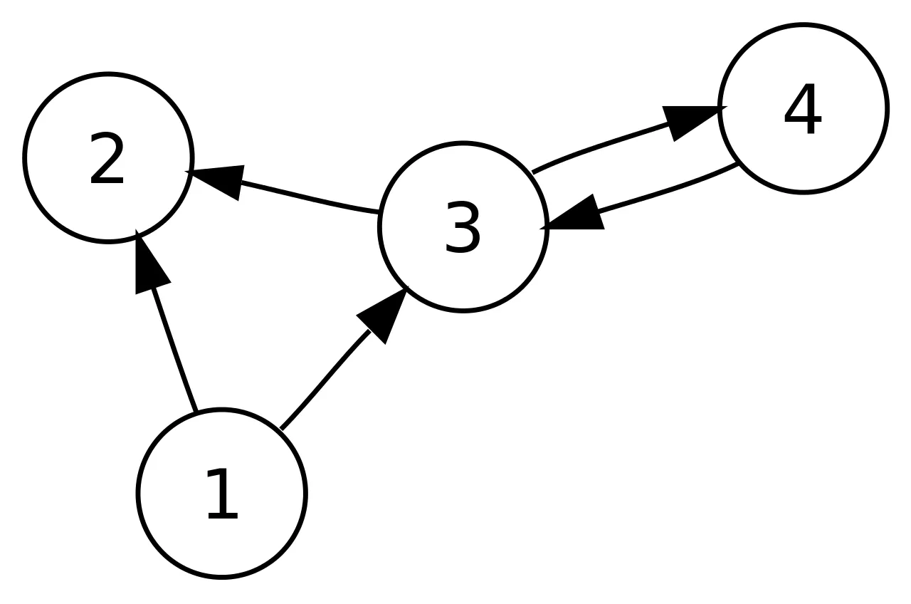
Data Structures and Algorithms(DSA) Tutorial

This article contains a detailed view of all common data structures and algorithms we use in our daily life programming to allow readers to become well equipped.

Listed below are the topics discussed in this article:

Introduction to Data Structures And Algorithms

- Linear Data Structures

- Hierarchical Data Structures

Algorithms

- Sorting Algorithms

- Searching Algorithms

Introduction

Data Structure is a way of collecting and organising data in such a way that we can perform operations on these data in an effective way. Data Structures is about rendering data elements in terms of some relationship, for better organization and storage. Let’s say We have some data which has, student’s name “Shivam” and his age 13. Here Shivam is of String data type and 13 is of integer data type.

In simple language, Data Structures are structures programmed to store ordered data, so that various operations can be performed on it easily. It represents the knowledge of data to be organized in memory. It should be designed and implemented in such a way that it reduces the complexity and increases the efficiency.

Basic types of Data Structures

As we have discussed above, anything that can store data can be called as a data structure, hence Integer, Float, Boolean, Char etc, all are data structures. They are known as Primitive Data Structures. Then we also have some complex Data Structures, which are used to store large and connected data. Some examples of Abstract Data Structure are Linked List, Stack, Queue, Tree, Graph etc.

All these data structures allow us to perform different operations on data. We select these based on our requirements.

Let’s Check out each of them in detail.

Linear Data Structures And Algorithms

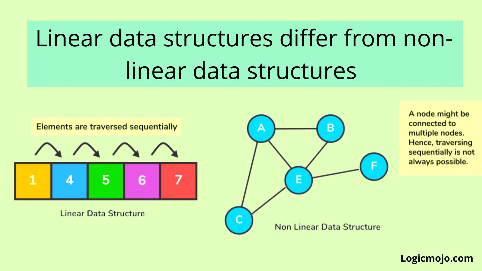
Linear data structures are those whose elements are in sequential and in ordered way. For example: Array, Linked list

Arrays

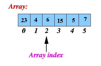
An array is a linear data structure representing a group of similar elements, accessed by index. Some Properties of Array Data Structures:

✔ ✔ Each element in an array is of the same data type and has the same size.

✔ ✔ Elements of the array are stored at contiguous memory locations with the first element starting at the smallest memory location.

✔ ✔ Elements of the array can be randomly accessed like arr[0] for the 1st element, arr[3] for the 3rd element.

✔ ✔ Array data structures are not completely dynamic, meaning memory is allocated as soon as the array is declared. However, we can create dynamic arrays using different libraries in many modern programming languages.

Linked List

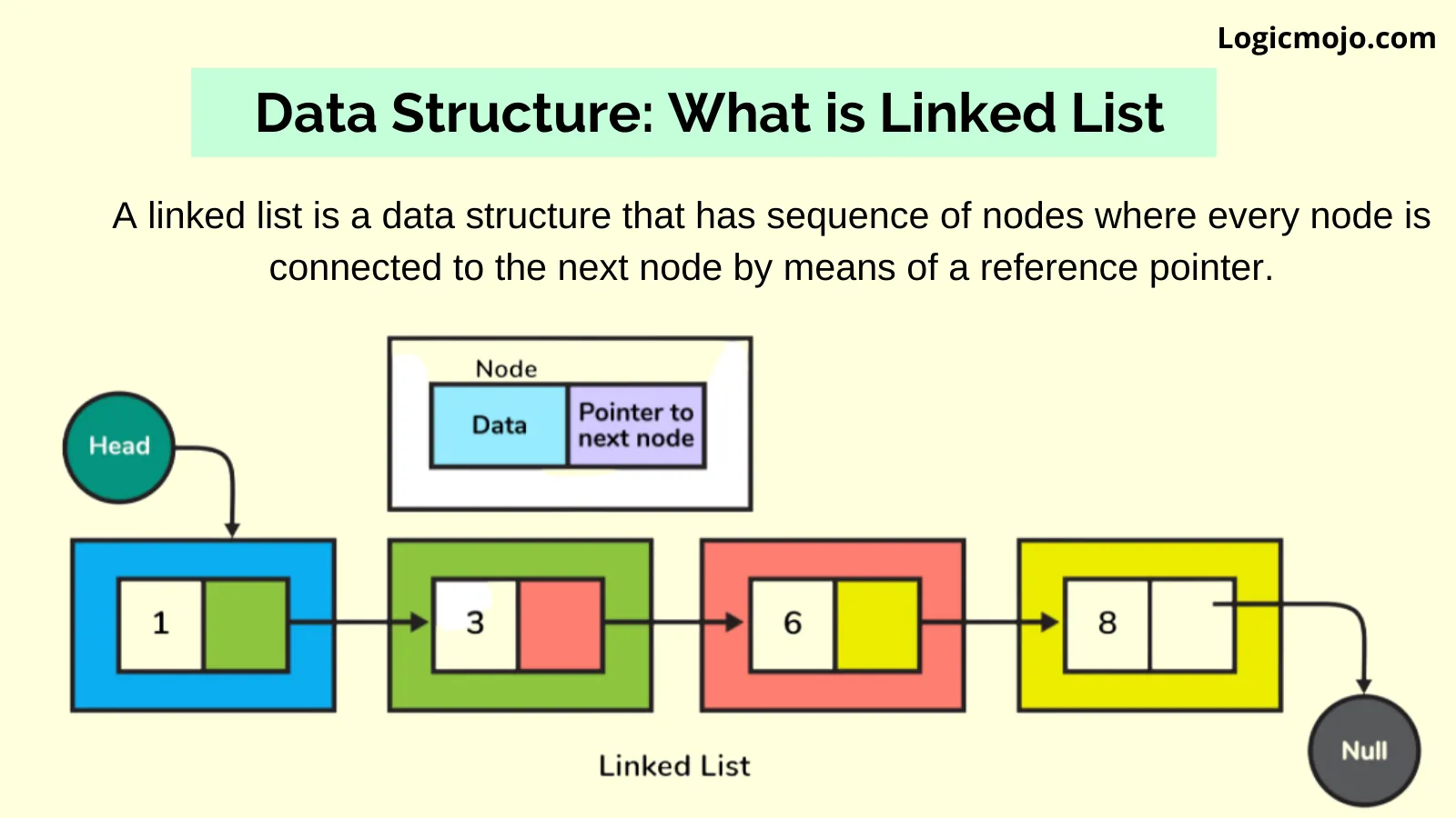
A linked list is a linear data structure with the collection of multiple nodes, where each element stores its own data and a pointer to the location of the next element. The last link of linked List points to null.

An element in Linked List is called node. The first node is called head. The last node is called tail.

Types of Linked List

Singly Linked List (Uni-directional)

The singly linked list is a linear data structure in which each element of the list contains a pointer which points to the next element in the list. Each node has two components: data and a pointer next which point to the next node in the list.

Below the Single LinkedList Creation Animation

        
    
    class LinkedList {
        Node head; // head of the list
        /* Linked list Node*/
        class Node {
            int data;
            Node next;
            // Constructor to create a new node
            // Next is by default initialized
            // as null
            Node(int d) { data = d; }
        }
    }
    
    

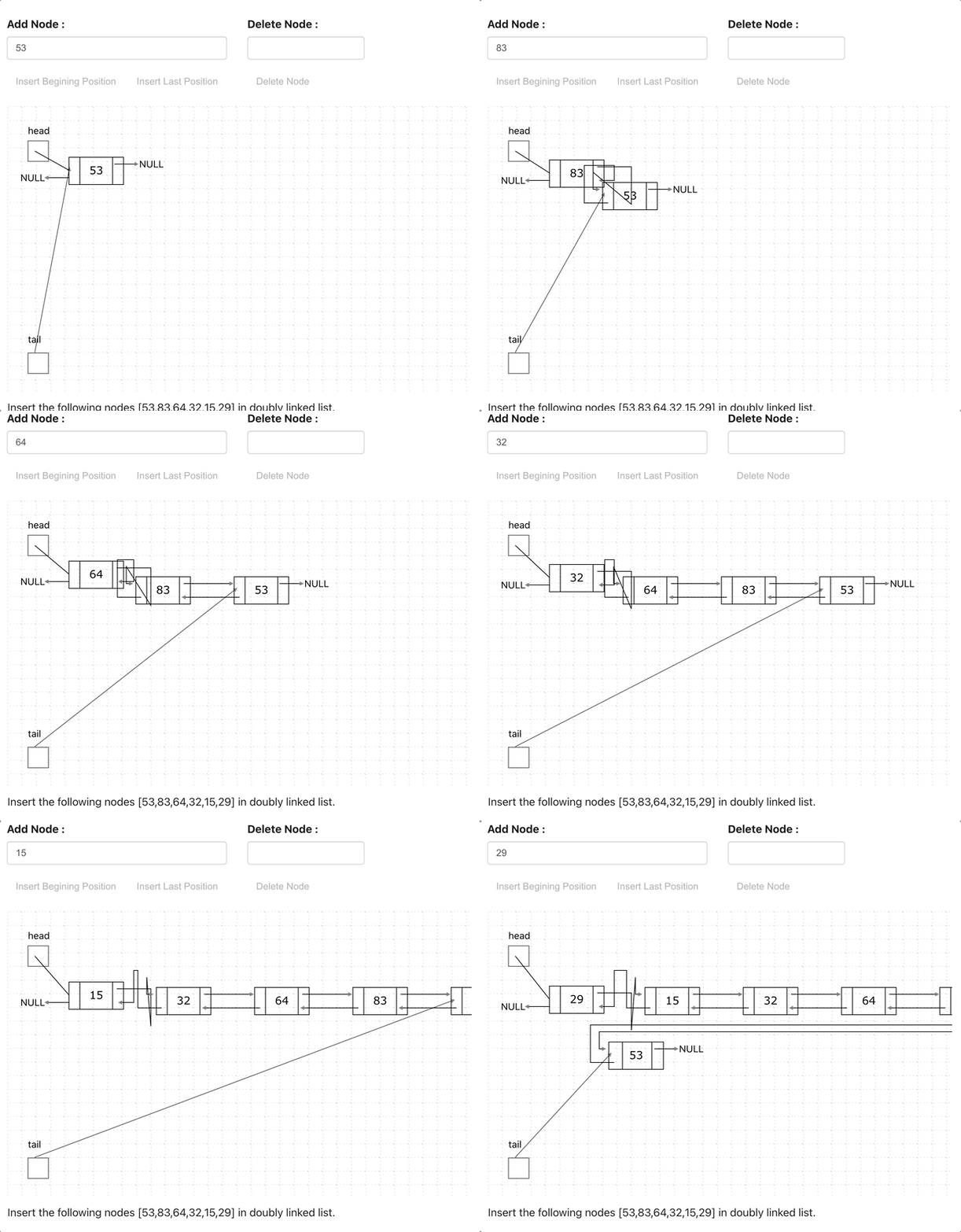
Doubly Linked List (Bi-Directional)

Doubly Linked List is just same as singly Linked List except it contains an extra pointer, typically called previous pointer, together with next pointer and data.

    
// Class for Doubly Linked List
public class DLL {
    Node head; // head of list
 
    /* Doubly Linked list Node*/
    class Node {
        int data;
        Node prev;
        Node next;
 
        // Constructor to create a new node
        // next and prev is by default initialized as null
        Node(int d) { data = d; }
    }
}

Advantages over singly linked list

✔ ✔A DLL can be traversed in both forward and backward direction.

✔ ✔The delete operation in DLL is more efficient if pointer to the node to be deleted is given.

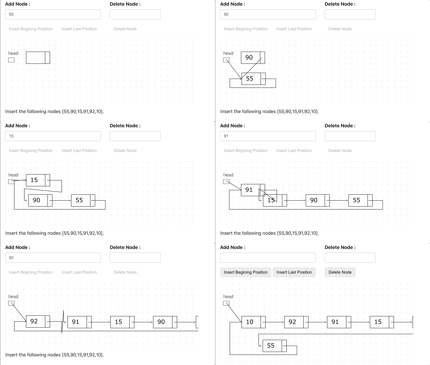
Circular Linked List

A circular linked list is a variation of a linked list in which the last node points to the first node, completing a full circle of nodes. You can say it doesn’t have null element at the end.

Application of Circular Linked List

✔ ✔The real life application where the circular linked list is used is our Personal Computers, where multiple applications are running. All the running applications are kept in a circular linked list and the OS gives a fixed time slot to all for running. The Operating System keeps on iterating over the linked list until all the applications are completed.

✔ ✔Another example can be Multiplayer games. All the Players are kept in a Circular Linked List and the pointer keeps on moving forward as a player's chance ends.

✔ ✔Circular Linked List can also be used to create Circular Queue. In a Queue we have to keep two pointers, FRONT and REAR in memory all the time, where as in Circular Linked List, only one pointer is required.

Stacks

What is Stack?

Stack, an abstract data structure, is a collection of objects that are inserted and removed according to the last-in-first-out (LIFO) principle. Objects can be inserted into a stack at any point of time, but only the most recently inserted (that is, “last”) object can be removed at any time.

Listed below are properties of a stack:

✔ ✔It is an orderd list in which insertion and deletion can be performed only at one end that is called the top.

✔ ✔Recursive data structure with a pointer to its top element.

✔ ✔Follows the last-in-first-out (LIFO) principle

Stack Concepts

✔ ✔When an element is inserted in a stack, the concept is called a push.

✔ ✔When an element is removed from the stack, the concept is called pop.

✔ ✔Trying to pop out an empty stack is called underflow (treat as Exception).

✔ ✔Trying to push an element in a full stack is called overflow (treat as Exception).

Applications of Stack

Following are some of the applications in which stacks play an important role.

✔Balancing of symbols

✔Page-visited history in a Web browser [Back Buttons]

✔Undo sequence in a text editor

✔Finding of spans (finding spans in stock markets)

Stack Implementation using Array

Push Operation

✔In a push operation, we add an element into the top of the stack.

✔Increment the variable Top so that it can now refer to the next memory location.

✔Add an element at the position of the incremented top.

✔This is referred to as adding a new element at the top of the stack.

✔Throw an exception if Stack is full.

public void push(int data) throws Exception {
    if (size() == capacity)
        throw new Exception("Stack is full.");
        stackArray[++top] = data;
}

Pop Operation

✔Remove the top element from the stack and decrease the size of a top by 1.

✔Throw an exception if Stack is empty.

public int pop() throws Exception {
    int data;
    if (isEmpty())
        throw new Exception("Stack is empty.");
    data = stackArray[top];
    stackArray[top--] = Integer.MIN_VALUE;
    return data;
}

Complexity Analysis

Let n be the number of elements in the stack. The complexities of stack operations with this representation can be given as:

✔Time Complexity of push() O(1)

✔Time Complexity of pop() O(1)

✔Space Complexity O(n)

Queues

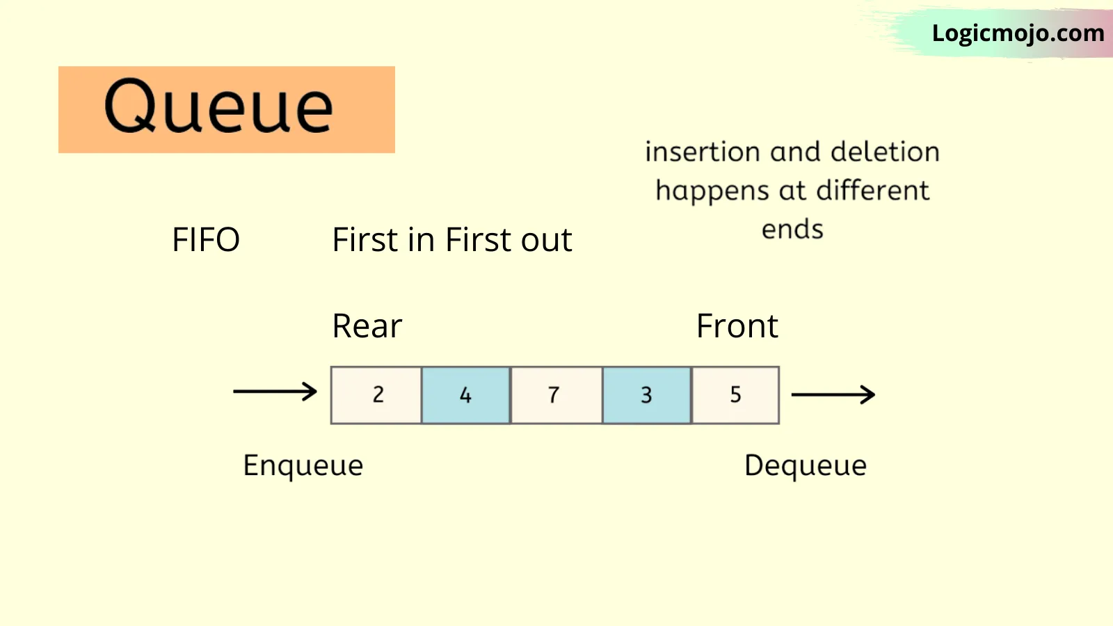
Queues are also another type of abstract data structure. Unlike a stack, the queue is a collection of objects that are inserted and removed according to the first-in-first-out (FIFO) principle.

Listed below are properties of a queue:

✔Often referred to as the first-in-first-out list

✔Supports two most fundamental methods enqueue(e): Insert element e, at the rear of the queue dequeue(): Remove and return the element from the front of the queue

Queue Concepts

✔When an element is inserted in a queue, the concept is called EnQueue.

✔When an element is removed from the queue, the concept is called DeQueue.

✔DeQueueing an empty queue is called underflow (treat as Exception)

✔EnQueuing an element in a full queue is called overflow (treat as Exception).

Applications of Queue

✔Operating systems schedule jobs (with equal priority) in the order of arrival (e.g., a print queue).

✔Simulation of real-world queues such as lines at a ticket counter, or any other first come the first-served scenario requires a queue.

✔Multiprogramming. Asynchronous data transfer (file IO, pipes, sockets).

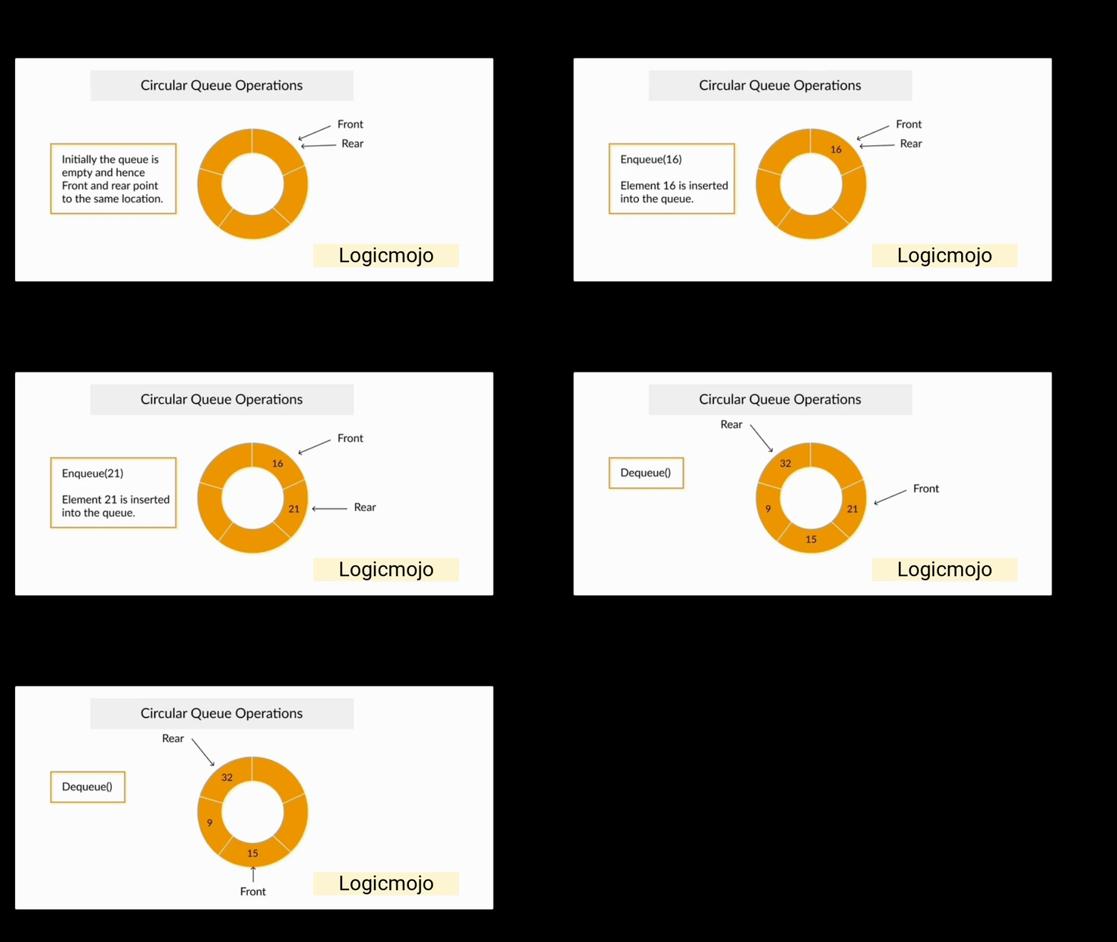
Implementation of Circular Queue using Linked List

Operations on Circular Queue:

For enQueue

✔Create a new node dynamically and insert value into it

✔Check if front==NULL, if it is true then front = rear = (newly created node)

✔If it is false then rear=(newly created node) and rear node always contains the address of the front node.

For Dequeue

✔Check whether queue is empty or not means front == NULL.

✔If it is empty then display Queue is empty. If queue is not empty then step 3

✔Check if (front==rear) if it is true then set front = rear = NULL else move the front forward in queue, update address of front in rear node and return the element.

Below is the code implementation in Java

// Java program for insertion and
// deletion in Circular Queue Using Linked List
import java.util.*;

class Solution {

  // Structure of a Node
  static class Node {
    int data;
    Node link;
  }

  static class Queue {
    Node front, rear;
  }

  // Function to create Circular queue
  static void enQueue(Queue q, int value)
  {
    Node temp = new Node();
    temp.data = value;
    if (q.front == null)
      q.front = temp;
    else
      q.rear.link = temp;

    q.rear = temp;
    q.rear.link = q.front;
  }

  // Function to delete element from Circular Queue
  static int deQueue(Queue q)
  {
    if (q.front == null) {
      System.out.printf("Queue is empty");
      return Integer.MIN_VALUE;
    }

    // If this is the last node to be deleted
    int value; // Value to be dequeued
    if (q.front == q.rear) {
      value = q.front.data;
      q.front = null;
      q.rear = null;
    }
    else // There are more than one nodes
    {
      Node temp = q.front;
      value = temp.data;
      q.front = q.front.link;
      q.rear.link = q.front;
    }

    return value;
  }

  // Function displaying the elements of Circular Queue
  static void displayQueue(Queue q)
  {
    Node temp = q.front;
    System.out.printf("\nElements in Circular Queue are: ");
    while (temp.link != q.front) {
      System.out.printf("%d ", temp.data);
      temp = temp.link;
    }
    System.out.printf("%d", temp.data);
  }

  /* Driver of the program */
  public static void main(String args[])
  {
    // Create a queue and initialize front and rear
    Queue q = new Queue();
    q.front = q.rear = null;

    // Inserting elements in Circular Queue
    enQueue(q, 14);
    enQueue(q, 22);
    enQueue(q, 6);

    // Display elements present in Circular Queue
    displayQueue(q);

    // Deleting elements from Circular Queue
    System.out.printf("\nDeleted value = %d", deQueue(q));
    System.out.printf("\nDeleted value = %d", deQueue(q));

    // Remaining elements in Circular Queue
    displayQueue(q);

    enQueue(q, 9);
    enQueue(q, 20);
    displayQueue(q);
  }
}

Hierarchical Data Structures And Algorithms in Java

Binary Tree

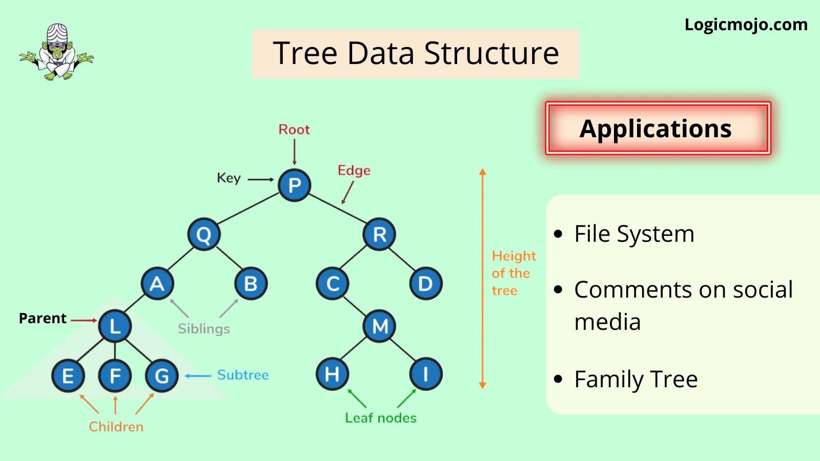
Binary Tree is a hierarchical tree data structures in which each node has at most two children, which are referred to as the left child and the right child. Each binary tree has the following groups of nodes:

Root Node: It is the topmost node and often referred to as the main node because all other nodes can be reached from the root

Left Sub-Tree, which is also a binary tree

Right Sub-Tree, which is also a binary tree

Binary Tree: Common Terminologies

Root:Topmost node in a tree.

Parent:Every node (excluding a root) in a tree is connected by a directed edge from exactly one other node. This node is called a parent.

Child:A node directly connected to another node when moving away from the root

Leaf/External node:Node with no children.

Internal node:Node with atleast one children.

Depth of a node:Number of edges from root to the node.

Height of a node:Number of edges from the node to the deepest leaf. Height of the tree is the height of the root

Listed below are the properties of a binary tree:

A binary tree can be traversed in two ways:

Depth First Traversal: In-order (Left-Root-Right), Preorder (Root-Left-Right) and Postorder (Left-Right-Root)

Breadth First Traversal: Level Order Traversal

Time Complexity of Tree Traversal: O(n)

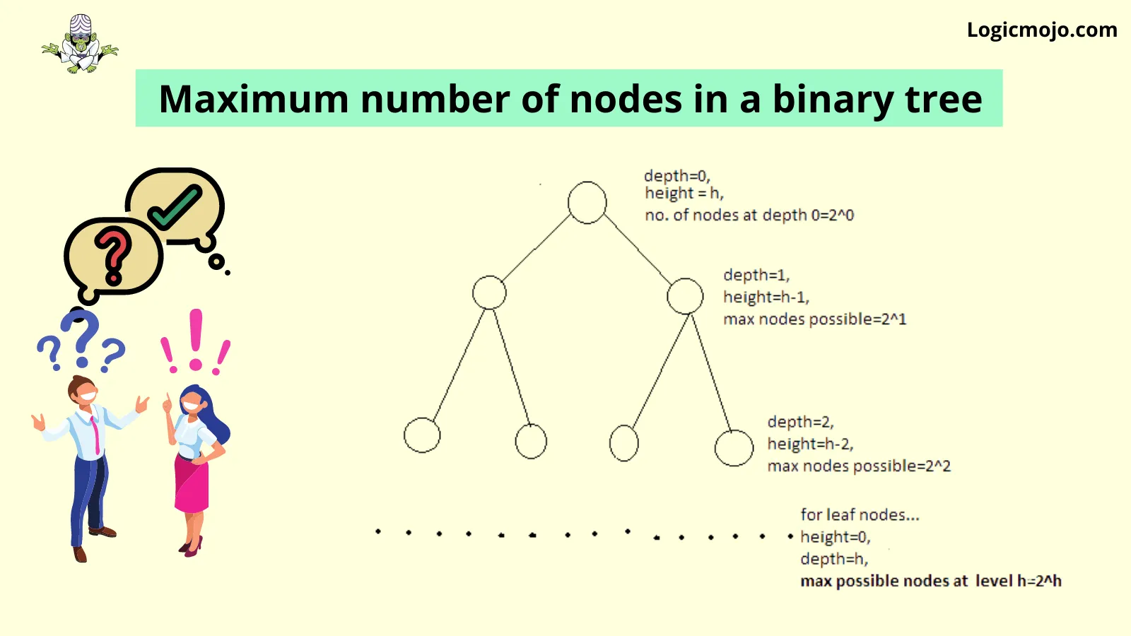
The maximum number of nodes at level "n" = 2^(n-1).

The maximum number of nodes of Binary Tree of height "h" = 2^(h).

Below is the image which gives better visualization that how maximum number of nodes of Binary tree is 2^(h)

Applications of binary trees include:

✔Used in many search applications where data is constantly entering/leaving

✔Used in almost every high-bandwidth router for storing router-tables

✔Used in compression algorithms and many more

Graph

What is graph (data structure)?

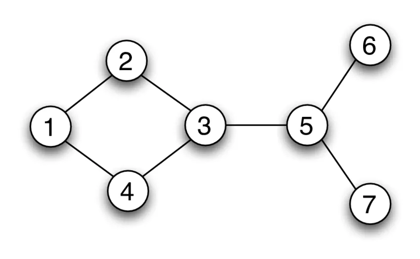
A graph is a common data structure that consists of a finite set of nodes (or vertices) and a set of edges connecting them.

A pair (x,y) is referred to as an edge, which communicates that the x vertex connects to the y vertex.

Graphs are used to solve real-life problems that involve representation of the problem space as a network. Examples of networks include telephone networks, circuit networks, social networks (like LinkedIn, Facebook etc.).

Types of graphs:

Undirected Graph:

In an undirected graph, nodes are connected by edges that are all bidirectional. For example if an edge connects node 1 and 2, we can traverse from node 1 to node 2, and from node 2 to 1.

Directed Graph:

In a directed graph, nodes are connected by directed edges – they only go in one direction. For example, if an edge connects node 1 and 2, but the arrow head points towards 2, we can only traverse from node 1 to node 2 – not in the opposite direction.

Types of Graph Representations:

Adjacency List

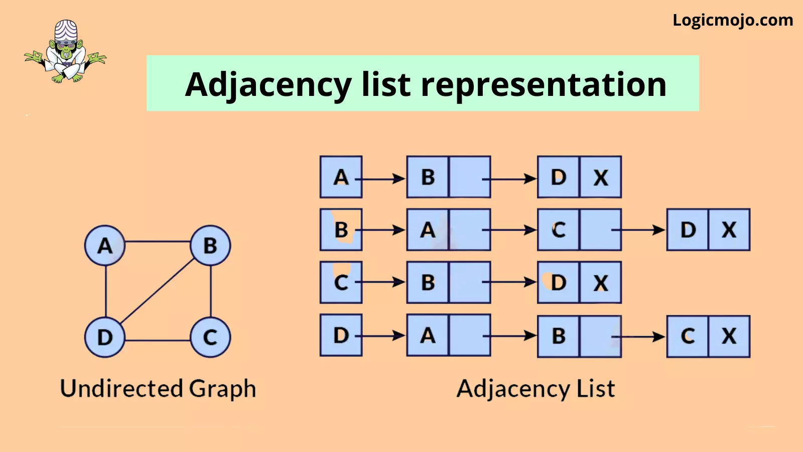
To create an Adjacency list, an array of lists is used. The size of the array is equal to the number of nodes. A single index, array[i] represents the list of nodes adjacent to the ith node.

For example, we have given below.

We use Java Collections to store the Array of Linked Lists.

class Graph{
    private int numVertices;
    private LinkedList<integer> adjLists[];
}

Adjacency Matrix

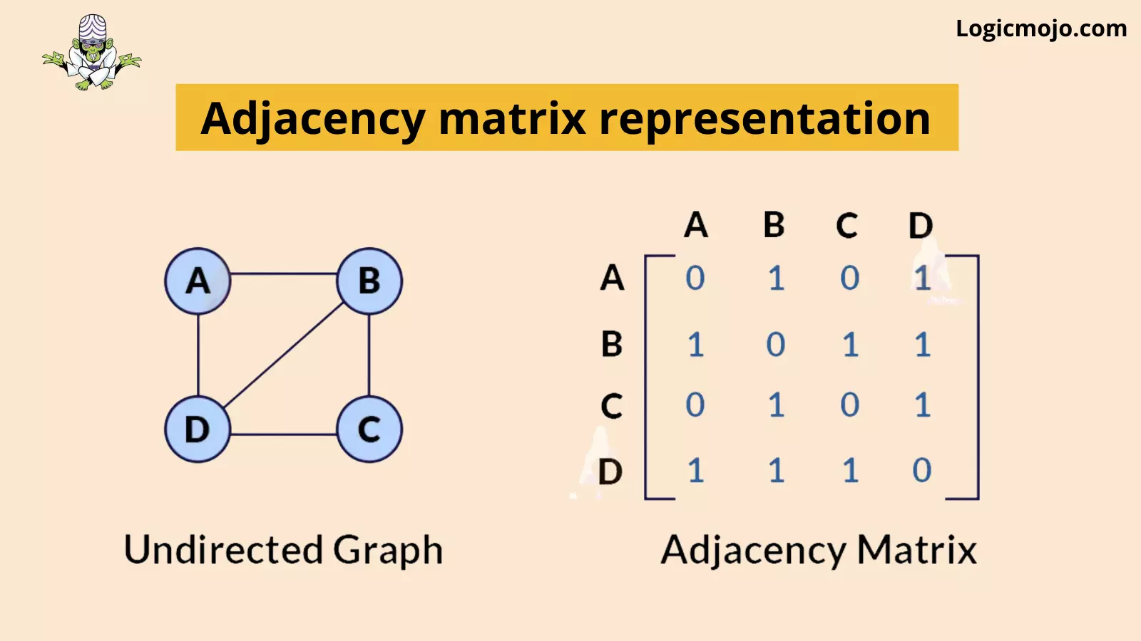
An Adjacency Matrix is a 2D array of size V x V where V is the number of nodes in a graph. A slot matrix[i][j] = 1 indicates that there is an edge from node i to node j.

For example, we have given below.

Here is the implementation part in Java.

public AdjacencyMatrix(int vertex){
        this.vertex = vertex;
        matrix = new int[vertex][vertex];
}

Algorithms in Java

Algorithms are deeply connected with computer science, and with data structures in particular. An algorithm is a sequence of instructions that describes a way of solving a specific problem in a finite period of time. They are represented in two ways:

Flowcharts- It is a visual representation of an algorithm’s control flow

Pseudocode– It is a textual representation of an algorithm that approximates the final source code

Note: The performance of the algorithm is measured based on time complexity and space complexity. Mostly, the complexity of any algorithm is dependent on the problem and on the algorithm itself.

Let’s explore the two major categories of algorithms in Java, which are:

Sorting Algorithms in Java

Sorting algorithms are algorithms that put elements of a list in a certain order. The most commonly used orders are numerical order and lexicographical order.

Let's dive into some famous sorting algorithms.

Bubble Sort in Java

Bubble Sort is a simple algorithm which is used to sort a given set of n elements provided in form of an array with n number of elements. Bubble Sort compares all the element one by one and sort them based on their values.

It is known as bubble sort, because with every complete iteration the largest element in the given array, bubbles up towards the last place or the highest index, just like a water bubble rises up to the water surface.

Here’s pseudocode representing Bubble Sort Algorithm (ascending sort context).

a[] is an array of size N
begin BubbleSort(a[])
 
declare integer i, j
for i = 0 to N - 1
   for j = 0 to N - i - 1
      if a[j] > a[j+1] then 
         swap a[j], a[j+1]
      end if
   end for
  return a
   
end BubbleSort

Worst and Average Case Time Complexity: O(n*n) (The worst-case occurs when an array is reverse sorted).

Best Case Time Complexity:O(n) (Best case occurs when an array is already sorted).

Selection Sort in Java

Selection sorting is a combination of both searching and sorting. The algorithm sorts an array by repeatedly finding the minimum element (considering ascending order) from the unsorted part and putting it at a proper position in the array.

Here’s pseudocode representing Selection Sort Algorithm (ascending sort context).

a[] is an array of size N
begin SelectionSort(a[])
 
 for i = 0 to n - 1
   /* set current element as minimum*/
      min = i    
      /* find the minimum element */
       for j = i+1 to n 
         if list[j] < list[min] then
            min = j;
         end if
      end for
  /* swap the minimum element with the current element*/
      if min != i  then
         swap list[min], list[i]
      end if
   end for
     
end SelectionSort

Time Complexity: O(n2) as there are two nested loops.

Auxiliary Space: O(1).

Insertion Sort in Java

Insertion Sort is a simple sorting algorithm which iterates through the list by consuming one input element at a time and builds the final sorted array. It is very simple and more effective on smaller data sets. It is stable and in-place sorting technique.

Here’s pseudocode representing Insertion Sort Algorithm (ascending sort context).

a[] is an array of size N
begin InsertionSort(a[])
 
for i = 1 to N
   key = a[ i ]
   j = i - 1
   while ( j >= 0 and a[ j ] > key0
      a[ j+1 ] = x[ j ]
      j = j - 1
   end while
   a[ j+1 ] = key
end for
 
end InsertionSort

Best Case: The best case is when input is an array that is already sorted. In this case insertion sort has a linear running time (i.e., Θ(n)).

Worst Case: The simplest worst case input is an array sorted in reverse order

QuickSort in Java

Quicksort algorithm is a fast, recursive, non-stable sort algorithm which works by the divide and conquer principle. It picks an element as pivot and partitions the given array around that picked pivot.

Here’s pseudocode representing Quicksort Algorithm.

QuickSort(A as array, low as int, high as int){
    if (low < high){
        pivot_location = Partition(A,low,high)
        Quicksort(A,low, pivot_location)
        Quicksort(A, pivot_location + 1, high)
    }
}
Partition(A as array, low as int, high as int){
     pivot = A[low]
     left = low
 
     for i = low + 1 to high{
         if (A[i] < pivot) then{
             swap(A[i], A[left + 1])
             left = left + 1
         }
     }
     swap(pivot,A[left])
 
    return (left)}

The complexity of quicksort in the average case is Θ(n log(n)) and in the worst case is Θ(n2).

Merge Sort in Java

Mergesort is a fast, recursive, stable sort algorithm which also works by the divide and conquer principle. Similar to quicksort, merge sort divides the list of elements into two lists. These lists are sorted independently and then combined. During the combination of the lists, the elements are inserted (or merged) at the right place in the list

Here’s pseudocode representing Merge Sort Algorithm

procedure MergeSort( a as array )
   if ( n == 1 ) return a
 
   var l1 as array = a[0] ... a[n/2]
   var l2 as array = a[n/2+1] ... a[n]
 
   l1 = mergesort( l1 )
   l2 = mergesort( l2 )
 
   return merge( l1, l2 )
end procedure
 
procedure merge( a as array, b as array )
 
   var c as array
   while ( a and b have elements )
      if ( a[0] > b[0] )
         add b[0] to the end of c
         remove b[0] from b
      else
         add a[0] to the end of c
         remove a[0] from a
      end if
   end while
    
   while ( a has elements )
      add a[0] to the end of c
      remove a[0] from a
   end while
    
   while ( b has elements )
      add b[0] to the end of c
      remove b[0] from b
   end while
    
   return c
     
end procedure

Searching Algorithms in Java

Searching is one of the most common and frequently performed actions in regular business applications. Search algorithms are algorithms for finding an item with specified properties among a collection of items. Let’s explore two of the most commonly used searching algorithms.

Linear Search Algorithm in Java

Linear search or sequential search is the simplest search algorithm. It involves sequential searching for an element in the given data structure until either the element is found or the end of the structure is reached. If the element is found, then the location of the item is returned otherwise the algorithm returns NULL.

Here’s pseudocode representing Linear Search in Java:

procedure linear_search (a[] , value)
for i = 0 to n-1
   if a[i] = value then
      print "Found "
      return i
   end if
print "Not found"
end for
 
end linear_search

It is a brute-force algorithm. While it certainly is the simplest, it’s most definitely is not the most common, due to its inefficiency. Time Complexity of Linear search is O(N).

Binary Search Algorithm in Java

Binary search, also known as logarithmic search, is a search algorithm that finds the position of a target value within an already sorted array. It divides the input collection into equal halves and the item is compared with the middle element of the list. If the element is found, the search ends there. Else, we continue looking for the element by dividing and selecting the appropriate partition of the array, based on if the target element is smaller or bigger than the middle element.

Here’s pseudocode representing Binary Search in Java:

Procedure binary_search
   a; sorted array
   n; size of array
   x; value to be searched
 
    lowerBound = 1
    upperBound = n 
 
   while x not found
      if upperBound < lowerBound 
         EXIT: x does not exists.
    
      set midPoint = lowerBound + ( upperBound - lowerBound ) / 2
       
      if A[midPoint] < x set lowerBound = midPoint + 1 if A[midPoint] > x
         set upperBound = midPoint - 1
 
      if A[midPoint] = x 
         EXIT: x found at location midPoint
   end while
    
end procedure

Binary Search Time Complexity

In each iteration, the search space is getting divided by 2. That means that in the current iteration you have to deal with half of the previous iteration array.

Best case could be the case where the first mid-value get matched to the element to be searched

Best Time Complexity: O(1)

Average Time Complexity: O(logn)

Worst Time Complexity: O(logn)

Since we are not using any space so space complexity will be O(1)

This brings us to the end of this ‘Data Structures and Algorithms in Java’ article. We have covered one of the most fundamental and important topics of Java. Hope you are clear with all that has been shared with you in this article.

Data Structures And Algorithms in Python

The knowledge of Data Structures and Algorithms forms the basis for identifying programmers, giving yet another reason for tech enthusiasts to get upscaled. While data structures help in the organization of data, algorithms help find solutions to the unending data analysis problems.

So, if you are still unaware of Data Structures and Algorithms in Python, here is a detailed article that will help you understand and implement them.

Before moving on, take a look at all the topics discussed in over here:

Introduction to Data Structures And Algorithms in Python

- Built in Data Structures

- User defined Data Structures

Algorithms in Python

- What are Algorithms?

- Elements of a Good Algorithms

- Sorting Algorithms

- Searching Algorithms

Introduction to Data Structures And Algorithms in Python

In-built Data Structures:

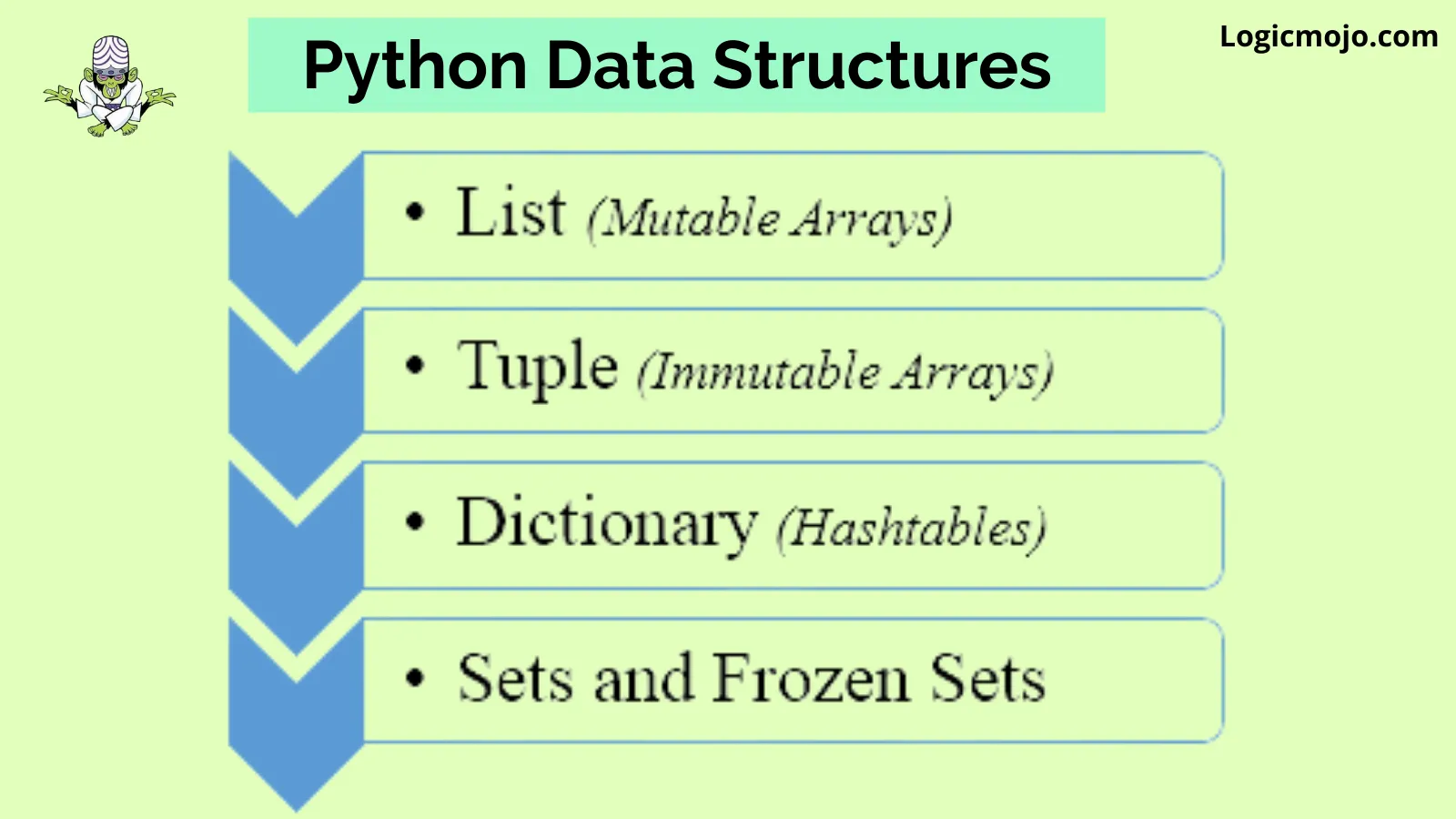
User-defined Data-structures And Algorithms in Python:

Linear Data Structures

Linear data structures in python are those whose elements are in sequential and in ordered way. For example: Linked list, Stack, Queue

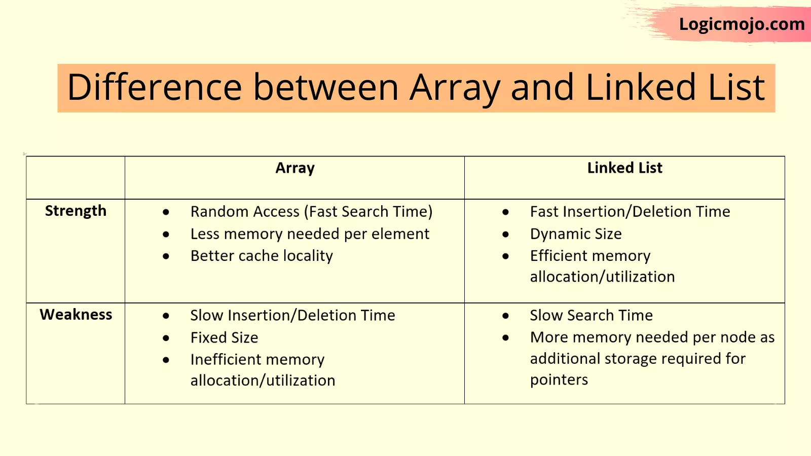
Linked List

A linked list is a linear data structure with the collection of multiple nodes, where each element stores its own data and a pointer to the location of the next element. The last link of linked List points to null.

An element in Linked List is called node. The first node is called head. The last node is called tail.

Types of Linked List

Singly Linked List (Uni-directional)

The singly linked list is a linear data structure in which each element of the list contains a pointer which points to the next element in the list. Each node has two components: data and a pointer next which point to the next node in the list.

# Node class
class Node:

  # Function to initialize the node object
  def __init__(self, data):
    self.data = data # Assign data
    self.next = None # Initialize
            # next as null

# Linked List class
class LinkedList:
  
  # Function to initialize the Linked
  # List object
  def __init__(self):
    self.head = None

Doubly Linked List (Bi-Directional)

Doubly Linked List is just same as singly Linked List except it contains an extra pointer, typically called previous pointer, together with next pointer and data.

# Node of a doubly linked list
class Node:
  def __init__(self, next=None, prev=None, data=None):
    self.next = next # reference to next node in DLL
    self.prev = prev # reference to previous node in DLL
    self.data = data

Advantages over singly linked list

✔A DLL can be traversed in both forward and backward direction.

✔The delete operation in DLL is more efficient if pointer to the node to be deleted is given.

Circular Linked List

A circular linked list is a variation of a linked list in which the last node points to the first node, completing a full circle of nodes. You can say it doesn’t have null element at the end.

Application of Circular Linked List

✔The real life application where the circular linked list is used is our Personal Computers, where multiple applications are running. All the running applications are kept in a circular linked list and the OS gives a fixed time slot to all for running. The Operating System keeps on iterating over the linked list until all the applications are completed.

✔Another example can be Multiplayer games. All the Players are kept in a Circular Linked List and the pointer keeps on moving forward as a player's chance ends.

✔Circular Linked List can also be used to create Circular Queue. In a Queue we have to keep two pointers, FRONT and REAR in memory all the time, where as in Circular Linked List, only one pointer is required.

Stacks

What is Stack?

Stack, an abstract data structure, is a collection of objects that are inserted and removed according to the last-in-first-out (LIFO) principle. Objects can be inserted into a stack at any point of time, but only the most recently inserted (that is, “last”) object can be removed at any time.

Listed below are properties of a stack:

✔It is an orderd list in which insertion and deletion can be performed only at one end that is called the top.

✔Recursive data structure with a pointer to its top element.

✔Follows the last-in-first-out (LIFO) principle

Stack Concepts

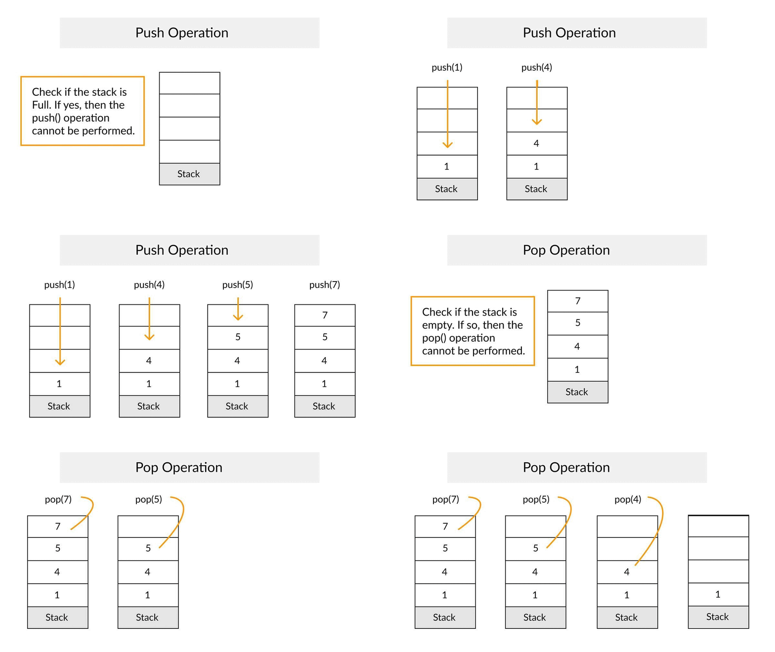
✔When an element is inserted in a stack, the concept is called a push.

✔When an element is removed from the stack, the concept is called pop.

✔Trying to pop out an empty stack is called underflow (treat as Exception).

✔Trying to push an element in a full stack is called overflow (treat as Exception).

Applications of Stack

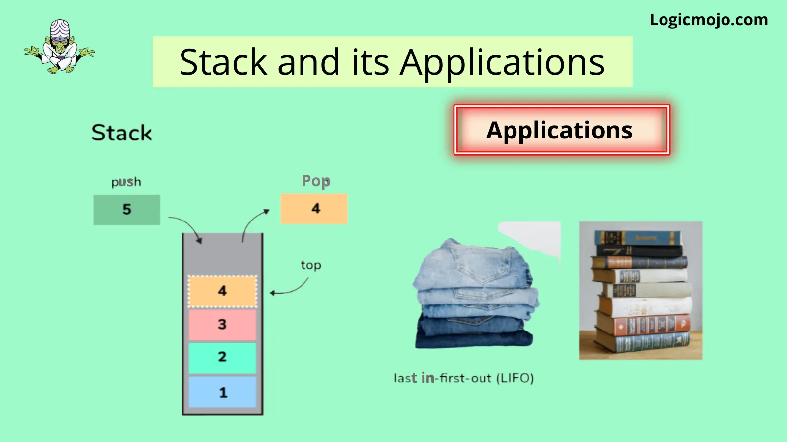
Following are some of the applications in which stacks play an important role.

✔Balancing of symbols

✔Page-visited history in a Web browser [Back Buttons]

✔Undo sequence in a text editor

✔Finding of spans (finding spans in stock markets)

Stack Implementation using List

Push Operation

✔ Write a class called Stack.

✔We have to maintain the data in a list. Let’s add an empty list in the Stack class with name elements.

✔To push the elements into the stack, we need a method. Let’s write a push method that takes data as an argument and append it to the elements list.

class Stack:
  def __init__(self):
    self.elements = []

  def push(self, data):
    self.elements.append(data)
    return data

Pop Operation

✔Similarly, let’s write the pop method that pops out the topmost element from the stack. We can use the pop method of the list data type.

class Stack:
  ## ...
  def pop(self):
    return self.elements.pop()

Complexity Analysis

Let n be the number of elements in the stack. The complexities of stack operations with this representation can be given as:

✔Time Complexity of push() O(1)

✔Time Complexity of pop() O(1)

✔Space Complexity O(n)

Queues

Queues are also another type of abstract data structure. Unlike a stack, the queue is a collection of objects that are inserted and removed according to the first-in-first-out (FIFO) principle.

Listed below are properties of a queue:

✔Often referred to as the first-in-first-out list

✔Supports two most fundamental methods enqueue(e): Insert element e, at the rear of the queue dequeue(): Remove and return the element from the front of the queue

Queue Concepts

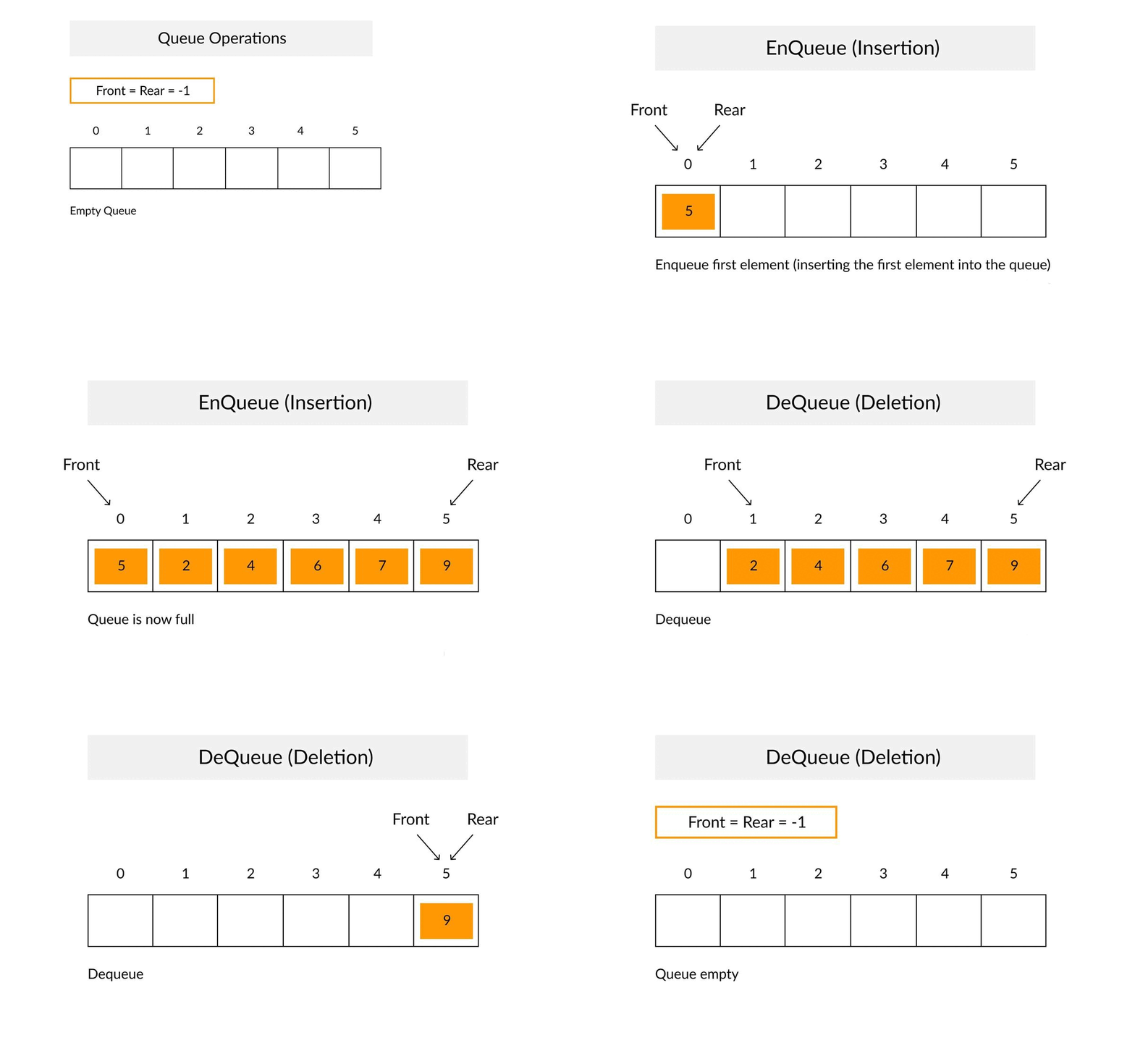
✔When an element is inserted in a queue, the concept is called EnQueue.

✔When an element is removed from the queue, the concept is called DeQueue.

✔DeQueueing an empty queue is called underflow (treat as Exception)

✔EnQueuing an element in a full queue is called overflow (treat as Exception).

Applications of Queue

✔Operating systems schedule jobs (with equal priority) in the order of arrival (e.g., a print queue).

✔Simulation of real-world queues such as lines at a ticket counter, or any other first come the first-served scenario requires a queue.

✔Multiprogramming. Asynchronous data transfer (file IO, pipes, sockets).

Implementation of Circular Queue using Linked List

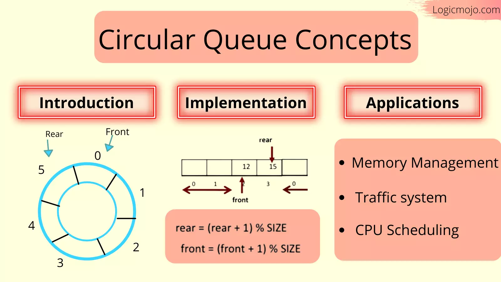
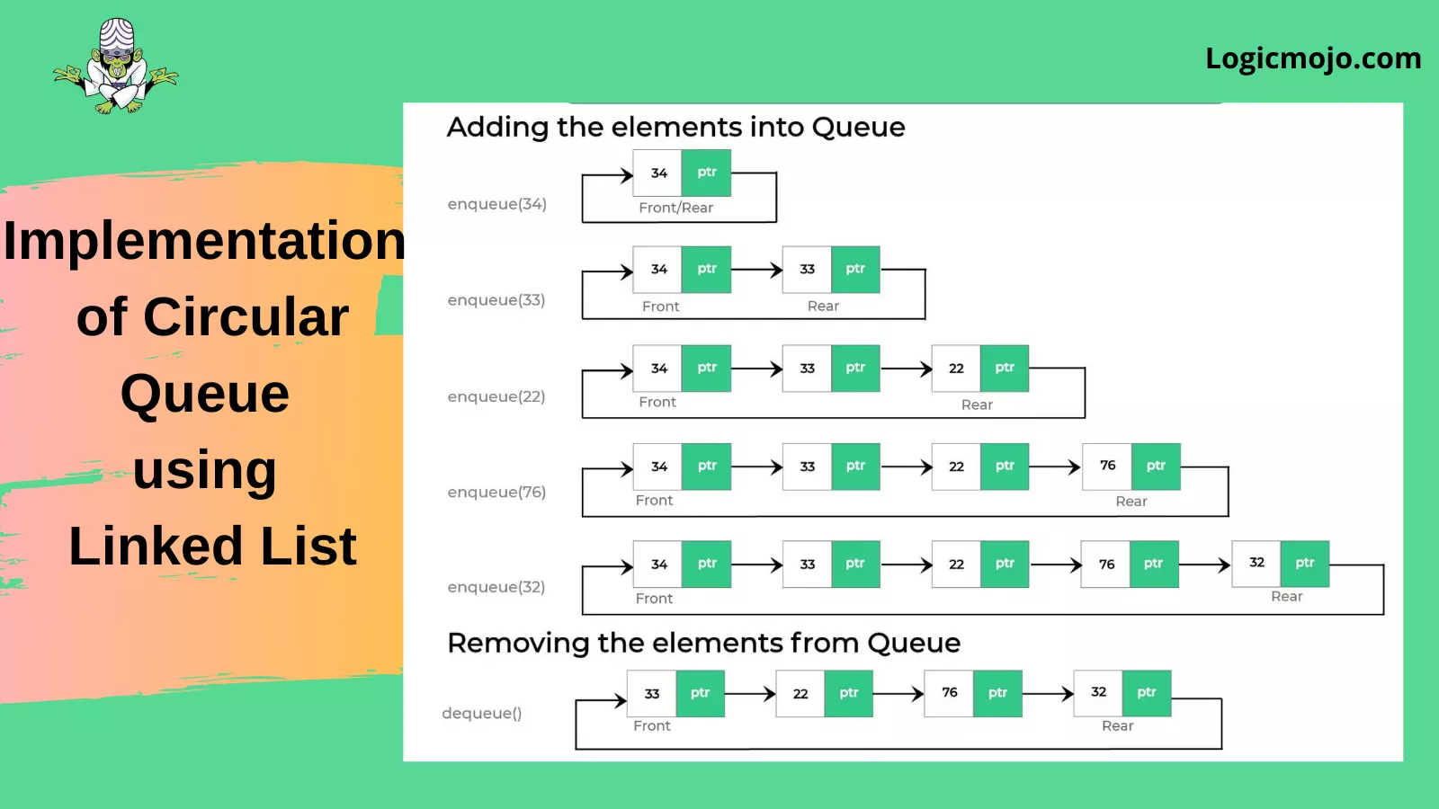
Operations on Circular Queue:

For enQueue

✔Create a new node dynamically and insert value into it

✔Check if front==NULL, if it is true then front = rear = (newly created node)

✔If it is false then rear=(newly created node) and rear node always contains the address of the front node.

For Dequeue

✔Check whether queue is empty or not means front == NULL.

✔If it is empty then display Queue is empty. If queue is not empty then step 3

✔Check if (front==rear) if it is true then set front = rear = NULL else move the front forward in queue, update address of front in rear node and return the element.

Below is the code implementation in Python

# Python3 program for insertion and
# deletion in Circular Queue

# Structure of a Node
class Node:
  def __init__(self):
    self.data = None
    self.link = None

class Queue:
  def __init__(self):
    front = None
    rear = None

# Function to create Circular queue
def enQueue(q, value):
  temp = Node()
  temp.data = value
  if (q.front == None):
    q.front = temp
  else:
    q.rear.link = temp

  q.rear = temp
  q.rear.link = q.front

# Function to delete element from
# Circular Queue
def deQueue(q):
  if (q.front == None):
    print("Queue is empty")
    return -999999999999

  # If this is the last node to be deleted
  value = None # Value to be dequeued
  if (q.front == q.rear):
    value = q.front.data
    q.front = None
    q.rear = None
  else: # There are more than one nodes
    temp = q.front
    value = temp.data
    q.front = q.front.link
    q.rear.link = q.front

  return value

# Function displaying the elements
# of Circular Queue
def displayQueue(q):
  temp = q.front
        print("Elements in Queue are:end="")
            
  while (temp.link != q.front):
    print(temp.data,end = " ")
    temp = temp.link
  print(temp.data)

# Driver Code
if __name__ == '__main__':

  # Create a queue and initialize
  # front and rear
  q = Queue()
  q.front = q.rear = None

  # Inserting elements in Circular Queue
  enQueue(q, 14)
  enQueue(q, 22)
  enQueue(q, 6)

  # Display elements present in
  # Circular Queue
  displayQueue(q)

  # Deleting elements from Circular Queue
  print("Deleted value = ", deQueue(q))
  print("Deleted value = ", deQueue(q))

  # Remaining elements in Circular Queue
  displayQueue(q)

  enQueue(q, 9)
  enQueue(q, 20)
  displayQueue(q)

Hierarchical Data Structures And Algorithms in Python

Binary Tree

Binary Tree is a hierarchical tree data structures in which each node has at most two children, which are referred to as the left child and the right child. Each binary tree has the following groups of nodes:

Root Node: It is the topmost node and often referred to as the main node because all other nodes can be reached from the root

Left Sub-Tree, which is also a binary tree

Right Sub-Tree, which is also a binary tree

Binary Tree: Common Terminologies

Root:Topmost node in a tree.

Parent:Every node (excluding a root) in a tree is connected by a directed edge from exactly one other node. This node is called a parent.

Child:A node directly connected to another node when moving away from the root

Leaf/External node:Node with no children.

Internal node:Node with atleast one children.

Depth of a node:Number of edges from root to the node.

Height of a node:Number of edges from the node to the deepest leaf. Height of the tree is the height of the root

Listed below are the properties of a binary tree:

A binary tree can be traversed in two ways:

Depth First Traversal: In-order (Left-Root-Right), Preorder (Root-Left-Right) and Postorder (Left-Right-Root)

Breadth First Traversal: Level Order Traversal

Time Complexity of Tree Traversal: O(n)

The maximum number of nodes at level "n" = 2^(n-1).

The maximum number of nodes of Binary Tree of height "h" = 2^(h).

Below is the image which gives better visualization that how maximum number of nodes of Binary tree is 2^(h)

Applications of binary trees include:

✔Used in many search applications where data is constantly entering/leaving

✔Used in almost every high-bandwidth router for storing router-tables

✔Used in compression algorithms and many more

Graph

What is graph (data structure)?

A graph is a common data structure that consists of a finite set of nodes (or vertices) and a set of edges connecting them.

A pair (x,y) is referred to as an edge, which communicates that the x vertex connects to the y vertex.

Graphs are used to solve real-life problems that involve representation of the problem space as a network. Examples of networks include telephone networks, circuit networks, social networks (like LinkedIn, Facebook etc.).

Types of graphs:

Undirected Graph:

In an undirected graph, nodes are connected by edges that are all bidirectional. For example if an edge connects node 1 and 2, we can traverse from node 1 to node 2, and from node 2 to 1.

Directed Graph:

In a directed graph, nodes are connected by directed edges – they only go in one direction. For example, if an edge connects node 1 and 2, but the arrow head points towards 2, we can only traverse from node 1 to node 2 – not in the opposite direction.

Types of Graph Representations:

Adjacency List

To create an Adjacency list, an array of lists is used. The size of the array is equal to the number of nodes. A single index, array[i] represents the list of nodes adjacent to the ith node.

For example, we have given below.

There is a reason Python gets so much love. A simple dictionary of vertices and its edges is a sufficient representation of a graph. You can make the vertex itself as complex as you want.

graph = {'A': set(['B', 'C']),
         'B': set(['A', 'D', 'E']),
         'C': set(['A', 'F']),
         'D': set(['B']),
         'E': set(['B', 'F']),
         'F': set(['C', 'E'])}

Adjacency Matrix

An Adjacency Matrix is a 2D array of size V x V where V is the number of nodes in a graph. A slot matrix[i][j] = 1 indicates that there is an edge from node i to node j.

For example, we have given below.

Here is the implementation part in Python.

# Adjacency Matrix representation in Python


class Graph(object):

    # Initialize the matrix
    def __init__(self, size):
        self.adjMatrix = []
        for i in range(size):
            self.adjMatrix.append([0 for i in range(size)])
        self.size = size

    # Add edges
    def add_edge(self, v1, v2):
        if v1 == v2:
            print("Same vertex %d and %d" % (v1, v2))
        self.adjMatrix[v1][v2] = 1
        self.adjMatrix[v2][v1] = 1
def main():
    g = Graph(5)
    g.add_edge(0, 1)
    g.add_edge(0, 2)
    g.add_edge(1, 2)
    g.add_edge(2, 0)
    g.add_edge(2, 3)

    g.print_matrix()


if __name__ == '__main__':
    main()

Algorithms:

Python algorithms are a set of instructions that are executed to get the solution to a given problem. Since algorithms are not language-specific, they can be implemented in several programming languages. No standard rules guide the writing of algorithms.

Elements of a Good Algorithm:

✔The steps need to be finite, clear and understandable

✔There should be a clear and precise description of inputs and outputs

✔Each step need to have a defined output that depends only on inputs in that step or the preceding steps

✔The algorithm should be flexible enough to mold it in order to allow a number of solutions

✔The steps should make use of general programming fundamentals and should not be language-specific

Let’s explore the two major categories of algorithms in Python, which are:

Sorting Algorithms in Python

Sorting algorithms are algorithms that put elements of a list in a certain order. The most commonly used orders are numerical order and lexicographical order.

Let's dive into some famous sorting algorithms.

Bubble Sort

Bubble Sort is a simple algorithm which is used to sort a given set of n elements provided in form of an array with n number of elements. Bubble Sort compares all the element one by one and sort them based on their values.

It is known as bubble sort, because with every complete iteration the largest element in the given array, bubbles up towards the last place or the highest index, just like a water bubble rises up to the water surface.

Here’s pseudocode representing Bubble Sort Algorithm (ascending sort context).

a[] is an array of size N
begin BubbleSort(a[])
 
declare integer i, j
for i = 0 to N - 1
   for j = 0 to N - i - 1
      if a[j] > a[j+1] then 
         swap a[j], a[j+1]
      end if
   end for
  return a
   
end BubbleSort

Worst and Average Case Time Complexity: O(n*n) (The worst-case occurs when an array is reverse sorted).

Best Case Time Complexity:O(n) (Best case occurs when an array is already sorted).

Selection Sort

Selection sorting is a combination of both searching and sorting. The algorithm sorts an array by repeatedly finding the minimum element (considering ascending order) from the unsorted part and putting it at a proper position in the array.

Here’s pseudocode representing Selection Sort Algorithm (ascending sort context).

a[] is an array of size N
begin SelectionSort(a[])
 
 for i = 0 to n - 1
   /* set current element as minimum*/
      min = i    
      /* find the minimum element */
       for j = i+1 to n 
         if list[j] < list[min] then
            min = j;
         end if
      end for
  /* swap the minimum element with the current element*/
      if min != i  then
         swap list[min], list[i]
      end if
   end for
     
end SelectionSort

Time Complexity: O(n2) as there are two nested loops.

Auxiliary Space: O(1).

Insertion Sort

Insertion Sort is a simple sorting algorithm which iterates through the list by consuming one input element at a time and builds the final sorted array. It is very simple and more effective on smaller data sets. It is stable and in-place sorting technique.

Here’s pseudocode representing Insertion Sort Algorithm (ascending sort context).

a[] is an array of size N
begin InsertionSort(a[])
 
for i = 1 to N
   key = a[ i ]
   j = i - 1
   while ( j >= 0 and a[ j ] > key0
      a[ j+1 ] = x[ j ]
      j = j - 1
   end while
   a[ j+1 ] = key
end for
 
end InsertionSort

Best Case: The best case is when input is an array that is already sorted. In this case insertion sort has a linear running time (i.e., Θ(n)).

Worst Case: The simplest worst case input is an array sorted in reverse order

QuickSort

Quicksort algorithm is a fast, recursive, non-stable sort algorithm which works by the divide and conquer principle. It picks an element as pivot and partitions the given array around that picked pivot.

Steps to implement Quick sort

Here’s pseudocode representing Quicksort Algorithm.

QuickSort(A as array, low as int, high as int){
    if (low < high){
        pivot_location = Partition(A,low,high)
        Quicksort(A,low, pivot_location)
        Quicksort(A, pivot_location + 1, high)
    }
}
Partition(A as array, low as int, high as int){
     pivot = A[low]
     left = low
 
     for i = low + 1 to high{
         if (A[i] < pivot) then{
             swap(A[i], A[left + 1])
             left = left + 1
         }
     }
     swap(pivot,A[left])
 
    return (left)}

The complexity of quicksort in the average case is Θ(n log(n)) and in the worst case is Θ(n2).

Merge Sort

Mergesort is a fast, recursive, stable sort algorithm which also works by the divide and conquer principle. Similar to quicksort, merge sort divides the list of elements into two lists. These lists are sorted independently and then combined. During the combination of the lists, the elements are inserted (or merged) at the right place in the list

Here’s pseudocode representing Merge Sort Algorithm

procedure MergeSort( a as array )
   if ( n == 1 ) return a
 
   var l1 as array = a[0] ... a[n/2]
   var l2 as array = a[n/2+1] ... a[n]
 
   l1 = mergesort( l1 )
   l2 = mergesort( l2 )
 
   return merge( l1, l2 )
end procedure
 
procedure merge( a as array, b as array )
 
   var c as array
   while ( a and b have elements )
      if ( a[0] > b[0] )
         add b[0] to the end of c
         remove b[0] from b
      else
         add a[0] to the end of c
         remove a[0] from a
      end if
   end while
    
   while ( a has elements )
      add a[0] to the end of c
      remove a[0] from a
   end while
    
   while ( b has elements )
      add b[0] to the end of c
      remove b[0] from b
   end while
    
   return c
     
end procedure

Searching Algorithms in Python

Searching is one of the most common and frequently performed actions in regular business applications. Search algorithms are algorithms for finding an item with specified properties among a collection of items. Let’s explore two of the most commonly used searching algorithms.

Linear Search Algorithm

Linear search or sequential search is the simplest search algorithm. It involves sequential searching for an element in the given data structure until either the element is found or the end of the structure is reached. If the element is found, then the location of the item is returned otherwise the algorithm returns NULL.

Here’s pseudocode representing Linear Search in Python:

procedure linear_search (a[] , value)
for i = 0 to n-1
   if a[i] = value then
      print "Found "
      return i
   end if
print "Not found"
end for
 
end linear_search

It is a brute-force algorithm. While it certainly is the simplest, it’s most definitely is not the most common, due to its inefficiency. Time Complexity of Linear search is O(N).

Binary Search Algorithm

Binary search, also known as logarithmic search, is a search algorithm that finds the position of a target value within an already sorted array. It divides the input collection into equal halves and the item is compared with the middle element of the list. If the element is found, the search ends there. Else, we continue looking for the element by dividing and selecting the appropriate partition of the array, based on if the target element is smaller or bigger than the middle element.

Here’s pseudocode representing Binary Search in Python:

Procedure binary_search
   a; sorted array
   n; size of array
   x; value to be searched
 
    lowerBound = 1
    upperBound = n 
 
   while x not found
      if upperBound < lowerBound 
         EXIT: x does not exists.
    
      set midPoint = lowerBound + ( upperBound - lowerBound ) / 2
       
      if A[midPoint] < x set lowerBound = midPoint + 1 if A[midPoint] > x
         set upperBound = midPoint - 1
 
      if A[midPoint] = x 
         EXIT: x found at location midPoint
   end while
    
end procedure

Binary Search Time Complexity

In each iteration, the search space is getting divided by 2. That means that in the current iteration you have to deal with half of the previous iteration array.

Best case could be the case where the first mid-value get matched to the element to be searched

Best Time Complexity: O(1)

Average Time Complexity: O(logn)

Worst Time Complexity: O(logn)

Since we are not using any space so space complexity will be O(1)

This brings us to the end of this ‘Data Structures and Algorithms in Python’ article. We have covered one of the most fundamental and important topics of Python. Hope you are clear with all that has been shared with you in this article.

Data Structures and Algorithms in C++

Knowing some fundamental data structures and algorithms both in theory and from a practical implementation perspective helps you in being a better C++ programmer, gives you a good foundation to understand standard library’s containers and algorithms inner “under the hood” mechanics, and serves as a kind of knowledge that is required in several coding interviews, as well.

In this article, Data Structures and Algorithms in C++, you’ll learn how to implement some fundamental data structures and algorithms in C++ from scratch, with a combination of theoretical introduction using animation, and practical C++ implementation code as well.

Before moving on, take a look at all the topics discussed in over here:

Introduction to Data Structures in C++

- Linear Data Structures

- Hierarchical Data Structures

- Algorithms in C++

- What are Algorithms?

- Elements of a Good Algorithms

- Sorting Algorithms

- Searching Algorithms

Introduction to Data Structures in C++

Data Structure is a way of collecting and organising data in such a way that we can perform operations on these data in an effective way. Data Structures is about rendering data elements in terms of some relationship, for better organization and storage. Let’s say We have some data which has, student’s name “Shivam” and his age 13. Here Shivam is of String data type and 13 is of integer data type.

In simple language, Data Structures are structures programmed to store ordered data, so that various operations can be performed on it easily. It represents the knowledge of data to be organized in memory. It should be designed and implemented in such a way that it reduces the complexity and increases the efficiency.

Linear Data Structures In C++

Linear data structures in C++ are those whose elements are in sequential and in ordered way. For example: Array, Linked list, etc

Arrays

An array is a linear data structure representing a group of similar elements, accessed by index. However, one shall not confuse array with the list like data structures in languages like python. Let us see arrays are presented in C++;

// simple declaration
int array[] = {1, 2, 3, 4, 5 };
// in pointer form (refers to an object stored in heap)
int * array = new int[5]; 

Note: However, we are accustomed to the more friendly vector data structure to which we can push without worrying about the size(i.e Dynamic Array).

Linked List

A linked list is a linear data structure with the collection of multiple nodes, where each element stores its own data and a pointer to the location of the next element. The last link of linked List points to null.

An element in Linked List is called node. The first node is called head. The last node is called tail.

Types of Linked List

Singly Linked List (Uni-directional)

The singly linked list is a linear data structure in which each element of the list contains a pointer which points to the next element in the list. Each node has two components: data and a pointer next which point to the next node in the list.

class Node {
public:
  int data;
  Node* next;
};

Doubly Linked List (Bi-Directional)

Doubly Linked List is just same as singly Linked List except it contains an extra pointer, typically called previous pointer, together with next pointer and data.

/* Node of a doubly linked list */
class Node
{
  public:
  int data;
  Node* next; // Pointer to next node in DLL
  Node* prev; // Pointer to previous node in DLL
};

Advantages over singly linked list

✔A DLL can be traversed in both forward and backward direction.

✔The delete operation in DLL is more efficient if pointer to the node to be deleted is given.

Circular Linked List

A circular linked list is a variation of a linked list in which the last node points to the first node, completing a full circle of nodes. You can say it doesn’t have null element at the end.

Application of Circular Linked List

✔The real life application where the circular linked list is used is our Personal Computers, where multiple applications are running. All the running applications are kept in a circular linked list and the OS gives a fixed time slot to all for running. The Operating System keeps on iterating over the linked list until all the applications are completed.

✔Another example can be Multiplayer games. All the Players are kept in a Circular Linked List and the pointer keeps on moving forward as a player's chance ends.

✔Circular Linked List can also be used to create Circular Queue. In a Queue we have to keep two pointers, FRONT and REAR in memory all the time, where as in Circular Linked List, only one pointer is required.

Stacks

What is Stack?

Stack, an abstract data structure, is a collection of objects that are inserted and removed according to the last-in-first-out (LIFO) principle. Objects can be inserted into a stack at any point of time, but only the most recently inserted (that is, “last”) object can be removed at any time.

Listed below are properties of a stack:

✔It is an orderd list in which insertion and deletion can be performed only at one end that is called the top.

✔Recursive data structure with a pointer to its top element.

✔Follows the last-in-first-out (LIFO) principle

Stack Concepts

✔When an element is inserted in a stack, the concept is called a push.

✔When an element is removed from the stack, the concept is called pop.

✔Trying to pop out an empty stack is called underflow (treat as Exception).

✔Trying to push an element in a full stack is called overflow (treat as Exception).

Applications of Stack

Following are some of the applications in which stacks play an important role.

✔Balancing of symbols

✔Page-visited history in a Web browser [Back Buttons]

✔Undo sequence in a text editor

✔Finding of spans (finding spans in stock markets)

Stack Implementation using Array

Push Operation

✔In a push operation, we add an element into the top of the stack.

✔Increment the variable Top so that it can now refer to the next memory location.

✔Add an element at the position of the incremented top.

✔This is referred to as adding a new element at the top of the stack.

✔Throw an exception if Stack is full.

void push(int val) {
   if(top>=n-1)
   cout<<"Stack Overflow"<<endl;
   else {
      top++;
      stack[top]=val;
   }
}

Pop Operation

✔Remove the top element from the stack and decrease the size of a top by 1.

✔Throw an exception if Stack is empty.

void pop() {
   if(top<=-1)
   cout<<"Stack Underflow"<<endl;
   else {
      cout<<"The popped element is "<< stack[top] <<endl;
      top--;
   }
}

Complexity Analysis

Let n be the number of elements in the stack. The complexities of stack operations with this representation can be given as:

✔Time Complexity of push() O(1)

✔Time Complexity of pop() O(1)

✔Space Complexity O(n)

Queues

Queues are also another type of abstract data structure. Unlike a stack, the queue is a collection of objects that are inserted and removed according to the first-in-first-out (FIFO) principle.

Listed below are properties of a queue:

✔Often referred to as the first-in-first-out list

✔Supports two most fundamental methods enqueue(e): Insert element e, at the rear of the queue dequeue(): Remove and return the element from the front of the queue

Queue Concepts

✔When an element is inserted in a queue, the concept is called EnQueue.

✔When an element is removed from the queue, the concept is called DeQueue.

✔DeQueueing an empty queue is called underflow (treat as Exception)

✔EnQueuing an element in a full queue is called overflow (treat as Exception).

Applications of Queue

✔Operating systems schedule jobs (with equal priority) in the order of arrival (e.g., a print queue).

✔Simulation of real-world queues such as lines at a ticket counter, or any other first come the first-served scenario requires a queue.

✔Multiprogramming. Asynchronous data transfer (file IO, pipes, sockets).

Implementation of Circular Queue using Linked List

Operations on Circular Queue:

For enQueue

✔Create a new node dynamically and insert value into it

✔Check if front==NULL, if it is true then front = rear = (newly created node)

✔If it is false then rear=(newly created node) and rear node always contains the address of the front node.

For Dequeue

✔Check whether queue is empty or not means front == NULL.

✔If it is empty then display Queue is empty. If queue is not empty then step 3

✔Check if (front==rear) if it is true then set front = rear = NULL else move the front forward in queue, update address of front in rear node and return the element.

Below is the code implementation in C++

// C++ program for insertion and
// deletion in Circular Queue
#include <bits/stdc++.h>
using namespace std;

// Structure of a Node
struct Node {
  int data;
  struct Node* link;
};

struct Queue {
  struct Node *front, *rear;
};

// Function to create Circular queue
void enQueue(Queue* q, int value)
{
  struct Node* temp = new Node;
  temp->data = value;
  if (q->front == NULL)
    q->front = temp;
  else
    q->rear->link = temp;

  q->rear = temp;
  q->rear->link = q->front;
}

// Function to delete element from Circular Queue
int deQueue(Queue* q)
{
  if (q->front == NULL) {
    printf("Queue is empty");
    return INT_MIN;
  }

  // If this is the last node to be deleted
  int value; // Value to be dequeued
  if (q->front == q->rear) {
    value = q->front->data;
    free(q->front);
    q->front = NULL;
    q->rear = NULL;
  }
  else // There are more than one nodes
  {
    struct Node* temp = q->front;
    value = temp->data;
    q->front = q->front->link;
    q->rear->link = q->front;
    free(temp);
  }

  return value;
}

// Function displaying the elements of Circular Queue
void displayQueue(struct Queue* q)
{
  struct Node* temp = q->front;
  printf("\nElements in Circular Queue are: ");
  while (temp->link != q->front) {
    printf("%d ", temp->data);
    temp = temp->link;
  }
  printf("%d", temp->data);
}

/* Driver of the program */
int main()
{
  // Create a queue and initialize front and rear
  Queue* q = new Queue;
  q->front = q->rear = NULL;

  // Inserting elements in Circular Queue
  enQueue(q, 14);
  enQueue(q, 22);
  enQueue(q, 6);

  // Display elements present in Circular Queue
  displayQueue(q);

  // Deleting elements from Circular Queue
  printf("\nDeleted value = %d", deQueue(q));
  printf("\nDeleted value = %d", deQueue(q));

  // Remaining elements in Circular Queue
  displayQueue(q);

  enQueue(q, 9);
  enQueue(q, 20);
  displayQueue(q);

  return 0;
}

Hierarchical Data Structures in C++

Binary Tree

Binary Tree is a hierarchical tree data structures in which each node has at most two children, which are referred to as the left child and the right child. Each binary tree has the following groups of nodes:

Root Node: It is the topmost node and often referred to as the main node because all other nodes can be reached from the root

Left Sub-Tree, which is also a binary tree

Right Sub-Tree, which is also a binary tree

Binary Tree: Common Terminologies

Root:Topmost node in a tree.

Parent:Every node (excluding a root) in a tree is connected by a directed edge from exactly one other node. This node is called a parent.

Child:A node directly connected to another node when moving away from the root

Leaf/External node:Node with no children.

Internal node:Node with atleast one children.

Depth of a node:Number of edges from root to the node.

Height of a node:Number of edges from the node to the deepest leaf. Height of the tree is the height of the root

Listed below are the properties of a binary tree:

A binary tree can be traversed in two ways:

Depth First Traversal: In-order (Left-Root-Right), Preorder (Root-Left-Right) and Postorder (Left-Right-Root)

Breadth First Traversal: Level Order Traversal

Time Complexity of Tree Traversal: O(n)

The maximum number of nodes at level "n" = 2^(n-1).

The maximum number of nodes of Binary Tree of height "h" = 2^(h).

Below is the image which gives better visualization that how maximum number of nodes of Binary tree is 2^(h)

Applications of binary trees include:

✔Used in many search applications where data is constantly entering/leaving

✔Used in almost every high-bandwidth router for storing router-tables

✔Used in compression algorithms and many more

Graph

What is graph (data structure)?

A graph is a common data structure that consists of a finite set of nodes (or vertices) and a set of edges connecting them.

A pair (x,y) is referred to as an edge, which communicates that the x vertex connects to the y vertex.

Graphs are used to solve real-life problems that involve representation of the problem space as a network. Examples of networks include telephone networks, circuit networks, social networks (like LinkedIn, Facebook etc.).

Types of graphs:

Undirected Graph:

In an undirected graph, nodes are connected by edges that are all bidirectional. For example if an edge connects node 1 and 2, we can traverse from node 1 to node 2, and from node 2 to 1.

Directed Graph:

In a directed graph, nodes are connected by directed edges – they only go in one direction. For example, if an edge connects node 1 and 2, but the arrow head points towards 2, we can only traverse from node 1 to node 2 – not in the opposite direction.

Types of Graph Representations:

Adjacency List

To create an Adjacency list, an array of lists is used. The size of the array is equal to the number of nodes. A single index, array[i] represents the list of nodes adjacent to the ith node.

For example, we have given below.

class Graph{
    int numVertices;
    list<int> *adjLists;
    
  public:
    Graph(int V);
    void addEdge(int src, int dest);
};

Adjacency Matrix

An Adjacency Matrix is a 2D array of size V x V where V is the number of nodes in a graph. A slot matrix[i][j] = 1 indicates that there is an edge from node i to node j.

For example, we have given below.

Here is the implementation part in C++.

#include<iostream>
using namespace std;
int vertArr[20][20]; //the adjacency matrix initially 0
int count = 0;
void displayMatrix(int v) {
   int i, j;
   for(i = 0; i < v; i++) {
      for(j = 0; j < v; j++) {
         cout << vertArr[i][j] << " ";
      }
      cout << endl;
   }
}
void add_edge(int u, int v) {       //function to add edge into the matrix
   vertArr[u][v] = 1;
   vertArr[v][u] = 1;
}
main(int argc, char* argv[]) {
   int v = 6;    //there are 6 vertices in the graph
   add_edge(0, 4);
   add_edge(0, 3);
   add_edge(1, 2);
   add_edge(1, 4);
   displayMatrix(v);
}

Algorithms:

Algorithms are a set of instructions that are executed to get the solution to a given problem. Since algorithms are not language-specific, they can be implemented in several programming languages. No standard rules guide the writing of algorithms.

Elements of a Good Algorithm:

✔The steps need to be finite, clear and understandable

✔There should be a clear and precise description of inputs and outputs

✔Each step need to have a defined output that depends only on inputs in that step or the preceding steps

✔The algorithm should be flexible enough to mold it in order to allow a number of solutions

✔The steps should make use of general programming fundamentals and should not be language-specific

Let’s explore the two major categories of algorithms in C++, which are:

Sorting Algorithms in C++

Sorting algorithms are algorithms that put elements of a list in a certain order. The most commonly used orders are numerical order and lexicographical order.

Let's dive into some famous sorting algorithms.

Bubble Sort

Bubble Sort is a simple algorithm which is used to sort a given set of n elements provided in form of an array with n number of elements. Bubble Sort compares all the element one by one and sort them based on their values.

It is known as bubble sort, because with every complete iteration the largest element in the given array, bubbles up towards the last place or the highest index, just like a water bubble rises up to the water surface.

Here’s pseudocode representing Bubble Sort Algorithm (ascending sort context).

a[] is an array of size N
begin BubbleSort(a[])
 
declare integer i, j
for i = 0 to N - 1
   for j = 0 to N - i - 1
      if a[j] > a[j+1] then 
         swap a[j], a[j+1]
      end if
   end for
  return a
   
end BubbleSort

Worst and Average Case Time Complexity: O(n*n) (The worst-case occurs when an array is reverse sorted).

Best Case Time Complexity:O(n) (Best case occurs when an array is already sorted).

Selection Sort

Selection sorting is a combination of both searching and sorting. The algorithm sorts an array by repeatedly finding the minimum element (considering ascending order) from the unsorted part and putting it at a proper position in the array.

Here’s pseudocode representing Selection Sort Algorithm (ascending sort context).

a[] is an array of size N
begin SelectionSort(a[])
 
 for i = 0 to n - 1
   /* set current element as minimum*/
      min = i    
      /* find the minimum element */
       for j = i+1 to n 
         if list[j] < list[min] then
            min = j;
         end if
      end for
  /* swap the minimum element with the current element*/
      if min != i  then
         swap list[min], list[i]
      end if
   end for
     
end SelectionSort

Time Complexity: O(n2) as there are two nested loops.

Auxiliary Space: O(1).

Insertion Sort

Insertion Sort is a simple sorting algorithm which iterates through the list by consuming one input element at a time and builds the final sorted array. It is very simple and more effective on smaller data sets. It is stable and in-place sorting technique.

Here’s pseudocode representing Insertion Sort Algorithm (ascending sort context).

a[] is an array of size N
begin InsertionSort(a[])
 
for i = 1 to N
   key = a[ i ]
   j = i - 1
   while ( j >= 0 and a[ j ] > key0
      a[ j+1 ] = x[ j ]
      j = j - 1
   end while
   a[ j+1 ] = key
end for
 
end InsertionSort

Best Case: The best case is when input is an array that is already sorted. In this case insertion sort has a linear running time (i.e., Θ(n)).

Worst Case: The simplest worst case input is an array sorted in reverse order

QuickSort

Quicksort algorithm is a fast, recursive, non-stable sort algorithm which works by the divide and conquer principle. It picks an element as pivot and partitions the given array around that picked pivot.

Steps to implement Quick sort

Here’s pseudocode representing Quicksort Algorithm.

QuickSort(A as array, low as int, high as int){
    if (low < high){
        pivot_location = Partition(A,low,high)
        Quicksort(A,low, pivot_location)
        Quicksort(A, pivot_location + 1, high)
    }
}
Partition(A as array, low as int, high as int){
     pivot = A[low]
     left = low
 
     for i = low + 1 to high{
         if (A[i] < pivot) then{
             swap(A[i], A[left + 1])
             left = left + 1
         }
     }
     swap(pivot,A[left])
 
    return (left)}

The complexity of quicksort in the average case is Θ(n log(n)) and in the worst case is Θ(n2).

Merge Sort

Mergesort is a fast, recursive, stable sort algorithm which also works by the divide and conquer principle. Similar to quicksort, merge sort divides the list of elements into two lists. These lists are sorted independently and then combined. During the combination of the lists, the elements are inserted (or merged) at the right place in the list

Here’s pseudocode representing Merge Sort Algorithm

procedure MergeSort( a as array )
   if ( n == 1 ) return a
 
   var l1 as array = a[0] ... a[n/2]
   var l2 as array = a[n/2+1] ... a[n]
 
   l1 = mergesort( l1 )
   l2 = mergesort( l2 )
 
   return merge( l1, l2 )
end procedure
 
procedure merge( a as array, b as array )
 
   var c as array
   while ( a and b have elements )
      if ( a[0] > b[0] )
         add b[0] to the end of c
         remove b[0] from b
      else
         add a[0] to the end of c
         remove a[0] from a
      end if
   end while
    
   while ( a has elements )
      add a[0] to the end of c
      remove a[0] from a
   end while
    
   while ( b has elements )
      add b[0] to the end of c
      remove b[0] from b
   end while
    
   return c
     
end procedure

Searching Algorithms in C++

Searching is one of the most common and frequently performed actions in regular business applications. Search algorithms are algorithms for finding an item with specified properties among a collection of items. Let’s explore two of the most commonly used searching algorithms.

Linear Search Algorithm

Linear search or sequential search is the simplest search algorithm. It involves sequential searching for an element in the given data structure until either the element is found or the end of the structure is reached. If the element is found, then the location of the item is returned otherwise the algorithm returns NULL.

Here’s pseudocode representing Linear Search in C++:

procedure linear_search (a[] , value)
for i = 0 to n-1
   if a[i] = value then
      print "Found "
      return i
   end if
print "Not found"
end for
 
end linear_search

It is a brute-force algorithm. While it certainly is the simplest, it’s most definitely is not the most common, due to its inefficiency. Time Complexity of Linear search is O(N).

Binary Search Algorithm

Binary search, also known as logarithmic search, is a search algorithm that finds the position of a target value within an already sorted array. It divides the input collection into equal halves and the item is compared with the middle element of the list. If the element is found, the search ends there. Else, we continue looking for the element by dividing and selecting the appropriate partition of the array, based on if the target element is smaller or bigger than the middle element.

Here’s pseudocode representing Binary Search in C++:

Procedure binary_search
   a; sorted array
   n; size of array
   x; value to be searched
 
    lowerBound = 1
    upperBound = n 
 
   while x not found
      if upperBound < lowerBound 
         EXIT: x does not exists.
    
      set midPoint = lowerBound + ( upperBound - lowerBound ) / 2
       
      if A[midPoint] < x set lowerBound = midPoint + 1 if A[midPoint] > x
         set upperBound = midPoint - 1
 
      if A[midPoint] = x 
         EXIT: x found at location midPoint
   end while
    
end procedure

Binary Search Time Complexity

In each iteration, the search space is getting divided by 2. That means that in the current iteration you have to deal with half of the previous iteration array.

Best case could be the case where the first mid-value get matched to the element to be searched

Best Time Complexity: O(1)

Average Time Complexity: O(logn)

Worst Time Complexity: O(logn)

Since we are not using any space so space complexity will be O(1)

This brings us to the end of this ‘Data Structures and Algorithms in C++’ article. We have covered one of the most fundamental and important topics of C++. Hope you are clear with all that has been shared with you in this article.

🚀Conclusion

We have now reached the end of this page. With the knowledge from this page, you should be able to answers your interview question confidently.