Introduction
A well-liked machine learning approach called decision trees may be applied to both classification and regression problems. They are the best option for students
in the area of machine learning since they are simple to comprehend, interpret, and use.
In machine learning, decision trees are a method for structuring the algorithm. The dataset features will be divided using a decision tree technique and a cost
function. Pruning, a method used to remove branches that could employ pointless features, is done on the decision tree before it is optimized. To lessen the danger
of overfitting or an extremely complicated tree, parameters like the decision tree's depth can also be modified.
The major part of machine learning decision trees will be applied to classification issues, classifying objects according to learnt attributes. The method can be
applied to regression issues or as a way to forecast continuous outcomes from unobserved data.
The key advantages of employing a decision tree in machine learning are its simplicity and ease of visualizing and comprehending the decision-making process.
Pruning the tree structure is frequently required because decision trees in machine learning can produce unnecessarily complicated branches by creating highly
granular branches.
We will go through every part of the decision tree algorithm in this complete guide including its underlying concepts, various decision tree kinds, how to design
a decision tree, and how to assess and improve a decision tree.
You will have a thorough grasp of decision trees at the end of this essay, as well as how to apply them to solve issues in the real world.
What Is a Decision Tree?
At its core, Decision tree machine learning is a versatile algorithm that uses a hierarchical structure resembling a tree to make decisions
or predictions based on input data. It is a supervised learning method that can be applied to both classification and regression tasks. The decision tree breaks
down the dataset into smaller and more manageable subsets, allowing us to navigate through the data and extract valuable insights.
Decision trees are a method of representing decisions and outcomes by mapping decisions in a branching structure. Decision trees are used to
estimate the likelihood that several iterations of decisions will be successful in achieving a certain objective. As a decision tree may be used to manually model
operational choices like a flowchart, the idea of a decision tree predates machine learning. They are often taught and used as a method of analyzing organizational
decision-making in the business, economics, and operation management fields.
Due to their ease of use and popularity in machine learning, decision trees are a common model structure. The model's decision-making process
is also easily understood because to the tree-like structure. The process of communicating a model's output to a human is a significant concern in machine learning.
It is frequently challenging to describe a given model's output since machine learning excels at task optimization without direct human input. A decision tree
structure makes it easier to understand the logic behind a model's decision-making process since each decision branch can be seen.
By learning basic decision rules inferred from past data (training data), a decision tree is used to generate a training model that may be used
to predict the class or value of the target variable. The decision tree might not always offer a simple solution or choice. Instead, it may provide the data
scientist choices so they can choose wisely on their own. Decision trees mimic human thought processes, making it typically simple for data scientists to comprehend
and evaluate the findings.
The CART algorithm, which stands for Classification and Regression Tree algorithm, is used to construct a decision tree.
It is a graphical depiction for obtaining all feasible answers to a choice or problem based on predetermined conditions. It is known as a
decision tree because, like a tree, it begins with the root node and grows on subsequent branches to form a structure like a tree. A decision tree only poses a
question and divides the tree into subtrees according to the response (Yes/No).
Numerous industries, including banking, healthcare, marketing, and engineering, frequently employ this method. Let's explore decision tree
machine learning in more detail with a practical example in order to assist you with understanding this concept.
Real-Life Example
Imagine you are a loan officer at a bank, and your task is to determine whether a loan applicant is likely to default or not. You have a dataset containing
information about previous loan applicants, including attributes such as age, income, employment status, credit score, and loan amount. Your goal is to build a
decision tree model that can accurately predict the likelihood of loan default.
To begin, you analyze the dataset and identify the target variable, which in this case is whether the loan applicant defaulted or not. This will serve as the basis
for making predictions. Next, you select the most relevant features from the dataset, such as income, credit score, and employment status, which can potentially
impact the loan repayment ability.
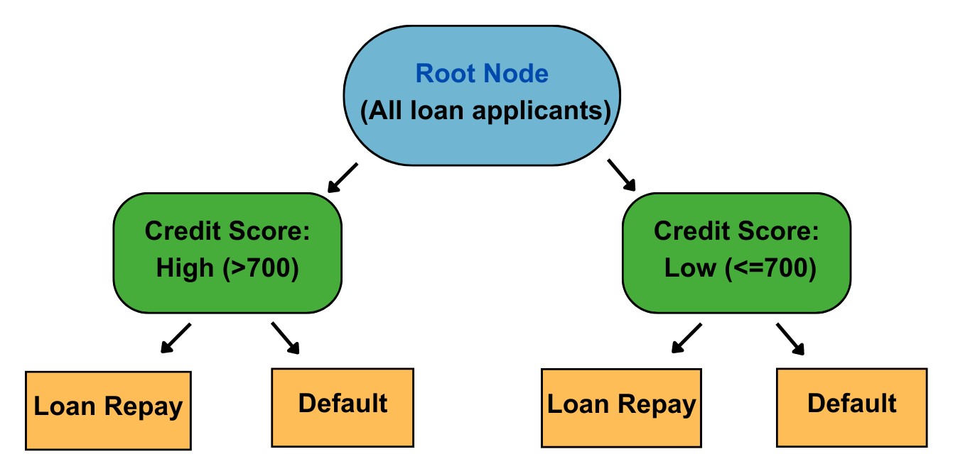
The decision tree algorithm starts with a root node, representing the entire dataset. It then evaluates different features to determine the best split that
maximizes the information gain or reduces the impurity in the data. For example, it may find that splitting the data based on credit score yields the highest
information gain.
The algorithm creates branches based on the credit score values, such as "high credit score" and "low credit score." Each branch represents a subset of the data
that satisfies the condition. It then continues recursively, evaluating different features at each internal node and splitting the data into smaller subsets based
on the selected features.
In our example, the decision tree may further split the data based on income and employment status. It may create branches such as "high income and employed,"
"low income and employed," and "unemployed." These branches represent different subsets of the data with distinct characteristics.
As the algorithm continues to split the data, it eventually reaches the leaves of the tree, which represent the final predictions or decisions. In our loan default
example, the leaves may represent "likely to default" and "likely to repay." The decision tree model has learned patterns and relationships within the dataset,
enabling it to make predictions on new loan applicants based on their attributes.
Now, when a new loan applicant comes in, you can input their information into the decision tree model. The model will traverse the tree, following the branches
based on the applicant's attributes, until it reaches a leaf node and provides a prediction whether the applicant is likely to default or not.
By using decision tree machine learning in this loan default scenario, you can effectively assess the risk associated with granting loans to different applicants.
This model provides transparency and interpretability, as you can trace the decision path within the tree and understand how various factors contribute to the final
prediction.
 Learn More️
What are different types of Decision Tree?
The majority of models are used in one of the two primary machine learning paradigms,
supervised or unsupervised machine learning. The state of the training
data and the issue the model is used to address are where these techniques diverge most from one another. The majority of the time, supervised machine learning
models are used to categorize items or data points, such as in facial recognition software, or to estimate continuous outcomes, such as in stock forecasting
tools. Unsupervised machine learning models are typically employed in automated recommendation systems to find association rules between variables or to cluster
data into groups of related data points.
The supervised kind of machine learning employs decision trees. Problems involving regression or classification may both be solved using this method.
Regression and classification trees are the two primary varieties of decision trees used in machine learning. Decision trees are mostly employed in machine
learning to handle classification difficulties, but they may also be used to address regression issues.
Depending on the kind of target variable we have, several decision trees can be used. It comes in two varieties:
1. Decision Tree using Categorical Variables:
A categorical variable decision tree is a decision tree with a categorical target variable.
2. Decision Tree of Continuous Variables:
If the decision tree's target variable is continuous, it is referred to as a continuous variable decision tree.
A continuous variable decision tree has the advantage that numerous factors may be used to predict the outcome as opposed to only one variable, as in a categorical
variable decision tree. Predictions are made using continuous variable decision trees. If the right method is used, the system may be applied to both linear and
non-linear interactions.
Classification Decision Tree
• In machine learning, decision trees are most frequently used to solve problems with classification. It is a supervised machine learning issue where the model is
trained to determine if the input data belongs to a specific class of objects. To categorize processed data, models are trained. In the training phase of the
machine learning model lifecycle, the model processes labelled training data to learn the classes.
• A model has to comprehend the characteristics that classify a data point into the various class labels in order to solve a classification issue. A categorization
issue might really arise in a variety of contexts. Document categorization, picture recognition software, and email spam detection are a few examples.
• A model for classifying objects or data can be organized using a classification tree. In a classification tree, the class labels are the leaves or endpoints of
the branches, the point at which the branches cease branching. The entire dataset is divided into smaller subgroups before the classification tree is gradually
created. When categorical or discrete target variables are involved, branching often takes place by binary partitioning. Each node, for instance, may branch
based on a yes or no response. When a target variable can be divided into one of two categories, such as yes or no, classification trees are utilized.
One category is where each branch ends.
Regression Decision Tree
• Regression problems occur when models are intended to anticipate or predict a continuous variable, such as forecasting changes in stock values or home
prices. It is a method for teaching a model how independent variables and a result relate to one another. Regression models are under the category of supervised
machine learning algorithms since they will be trained using labelled training data.
• Regression models for machine learning are developed to discover the link between output and input data. Once the connection has been established, the model may be
used to predict results from unknown input data. These models may be used to not only fill in the gaps in the historical data but also to forecast future or
emerging patterns in a variety of scenarios.Regression models may be used in machine learning for finance to predict future retail sales, property prices, or
portfolio performance.
Important Terms of a Decision Tree
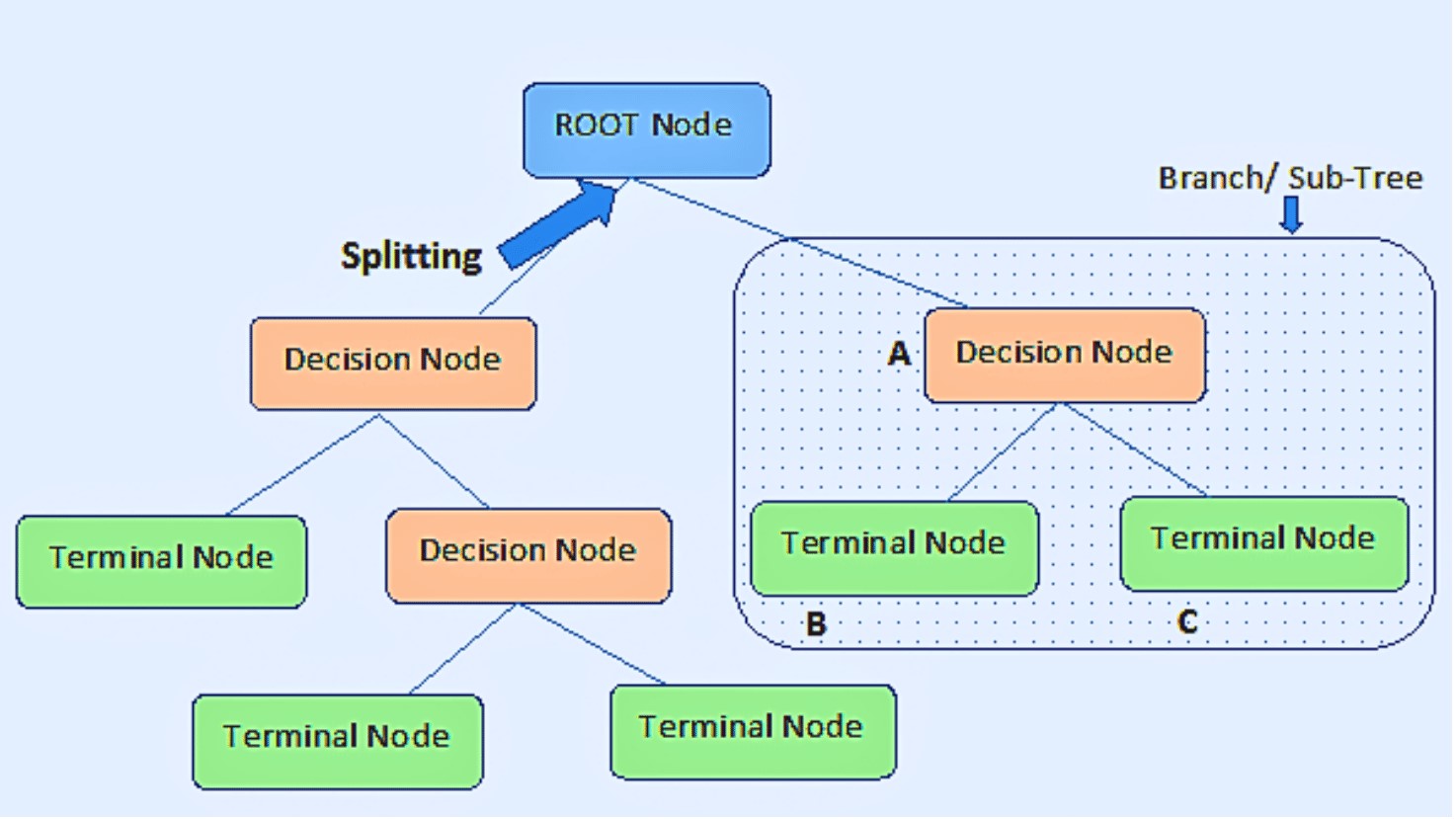
• Root node: It is the node at the very top of a decision tree, and it is from this node that the population begins to divide into groups based on
different attributes.
• Decision Nodes: Decision Node refers to the nodes obtained after separating the root nodes.
• Leaf Nodes: Leaf nodes or terminal nodes are the nodes where further splitting is not allowed.
• Splitting: It involves splitting a node into two or more smaller nodes.
• Subtree / Branch: Similar to how a tiny area of a graph is referred to as a sub-graph, this decision tree's sub-section is referred to as a sub-tree.
• Pruning: Pruning is the process of removing sub-nodes from a decision node. You might describe splitting in reverse.
• Child and Parent Node: A node that has sub-nodes is referred to as the parent node of the sub-nodes, whereas sub-nodes are the offspring of a parent node.
Why do we use Decision Trees?
When it comes to machine learning algorithms, choosing the right one for your specific dataset and problem is crucial. Decision trees offer
several compelling reasons for their usage, making them a popular choice in various domains. Let's delve into these reasons and explore them in more detail:
Mimicking Human Thinking: Decision trees are designed to mimic human thinking and decision-making processes. They are structured in a way that resembles the way
humans approach decision-making. By breaking down complex problems into smaller and more manageable steps, decision trees enable us to understand the underlying
logic behind the decision-making process. This makes them more intuitive and easier to interpret compared to other complex algorithms.
Interpretability: Decision trees provide a high level of interpretability. The tree-like structure of decision trees allows us to visualize and comprehend the
decision-making process in a clear and transparent manner. We can easily trace the path from the root node to the leaf nodes, understanding the conditions and
attributes that led to each decision or prediction. This interpretability is essential in various domains where explanations are required, such as finance,
healthcare, and legal systems.
Handling Nonlinear Relationships: Decision trees are well-suited for capturing nonlinear relationships between features and target variables. They can handle
complex datasets where the relationships between variables are not linear. Decision trees partition the data based on different features, creating branches that
represent distinct subsets of the data. This enables decision trees to capture nonlinear patterns and make accurate predictions or decisions based on these
patterns.
Feature Selection: Decision trees automatically perform feature selection as part of the training process. They evaluate the importance of different features by
considering their contribution to the decision-making process. Features that have a significant impact on the target variable are assigned higher importance, while
irrelevant features are given less importance. This feature selection capability reduces the dimensionality of the problem and focuses on the most relevant
attributes, leading to improved model performance and efficiency.
Handling Missing Values and Outliers: Decision trees can handle missing values and outliers in the data without significant preprocessing. Missing values can be
handled by assigning the majority class or the class with the highest frequency in the parent node. Outliers do not heavily affect the decision tree's performance,
as the algorithm works by splitting the data based on thresholds and conditions. This robustness to missing values and outliers makes decision trees a convenient
choice when dealing with real-world datasets that often contain imperfections.
Ensemble Methods: Decision trees can be combined using ensemble methods like random forests or gradient boosting. These techniques involve training multiple
decision trees and aggregating their predictions to make the final decision. Ensemble methods enhance the performance and robustness of decision tree models by
reducing overfitting and increasing generalization. They combine the strengths of individual decision trees to create a more accurate and reliable model.
The Methodology for Decision Trees
The notion of decision making based on conditions may be analyzed and shown graphically if given a problem to solve; the diagram will resemble an upside-down
tree with the root at the top and branches extending downwards.
What causes this? The root represents the starting point, where we have a collection of information or choices, which we examine using a few different criteria
before deciding what to do. In an inverted tree diagram, the root is known as the root node and the branches—known as the leaf nodes—represent the results of a
choice.
The diagrammatic technique aids in providing people with a visual explanation of the notion of probability and outcome. The number of layers would depend on the
number of conditions if we were to express it as 'IF... ELSE... IF' statements in pseudocode or plain English (using a programmatic method). To manage the numerous
iterations necessary to navigate through the complicated data, they are frequently in a nested or loop form.
How Does a Decision Tree Work?
In a decision tree, the algorithm begins at the root node and works its way up to forecast the class of the provided dataset. This algorithm follows the branch
and jumps to the following node by comparing the values of the root attribute with those of the record (actual dataset) attribute.
The algorithm verifies the attribute value with the other sub-nodes once again for the following node before continuing. It keeps doing this until it reaches the
tree's leaf node.
The kind of target variables is taken into consideration while choosing an algorithm. Let's examine some of the Decision Tree algorithms:
ID3: It is extension of D3, a shortened version of "Iterative Dichotomiser 3." Entropy and information gain are used by this technique as measures to assess potential
splits.
C4.5: This algorithm, which was created by Quinlan along with ID3, is regarded as its successor. Evaluation of split points inside the decision trees can be done using
information gain or gain ratios.
CART: CART is an acronym for "classification and regression trees". Gini impurity is often used by this method to choose the best characteristic to split on. A lower
number is preferable when using Gini impurity to evaluate.
CHAID: The term, CHAID, is an abbreviation for "Chi-square automatic interaction detection," which performs multi-level splits when computing classification trees.
The ID3 algorithm constructs decision trees by doing a top-down greedy search across the space of potential branches, with no backtracking. As the name implies,
a greedy algorithm always chooses the option that appears to be the best at the time.
Let's look into the inner workings of a decision tree and explore how it makes decisions. We'll cover the steps involved, the criteria for
splitting the data, and provide an example to illustrate the process.
A decision tree algorithm follows these main steps:
1. Selecting the Root Node: The decision tree starts with a root node, representing the entire dataset. This node contains all the available data points.
2. Choosing the Best Splitting Attribute: The algorithm evaluates different features and selects the best one to split the data. The splitting attribute is
chosen based on certain metrics, such as information gain or Gini impurity. These metrics quantify the homogeneity or impurity of the data, helping the algorithm
decide which feature to split on. Find the best attribute in the dataset using Attribute Selection Measure (ASM).
- Information Gain: Information gain measures the reduction in entropy or uncertainty achieved by splitting the data on a particular feature. Entropy, denoted
by H(S), represents the impurity of a set S.
Information gain = Entropy(parent) – [Weighted average] * Entropy(children)
- Gini Impurity: Gini impurity measures the probability of misclassifying a randomly chosen element in a set.
By calculating information gain or Gini impurity for each feature, the algorithm determines the best split that maximizes the gain or reduces the impurity.
3. Creating Branches and Nodes: Once the best splitting feature is determined, the algorithm creates child nodes or branches from the current node. Each
branch represents a possible value or outcome of the selected feature. The dataset is divided into subsets based on these branches, where each subset corresponds
to a specific branch.
4. Recursive Splitting: The splitting process continues recursively for each child node until a stopping criterion is met. This criterion could be reaching a
certain depth, achieving a minimum number of data points in a leaf node, or other predefined conditions.
5. Leaf Nodes and Predictions: When the recursive splitting process reaches the leaf nodes, these nodes represent the final predictions or decisions. For
classification tasks, the leaf nodes are assigned a class label based on the majority of data points belonging to a particular class. For regression tasks, the
leaf nodes may contain the average or mean value of the target variable.
• Now, let's illustrate this process with a simple example. Suppose we have a dataset of students with attributes like age, gender, and test scores. The task is to
predict whether a student will pass or fail the final exam.
• The decision tree algorithm starts by evaluating different features and selects age as the best splitting feature. It creates two branches: "age <= 10" and
"age > 10". Each branch represents a subset of the data based on the age criteria.
• For the branch "age <= 10", let's say all students pass the exam. In this case, we reach a leaf node with the prediction "pass".
• For the branch "age > 10", we further split the data based on another feature, such as gender. Let's assume that for males, 70% pass the exam and 30% fail, while
for females, 80% pass and 20% fail. These statistics guide the algorithm to create more branches and leaf nodes until reaching the desired depth or meeting the
stopping criteria.
• Once the decision tree is constructed, new data points can be traversed through the tree. For example, if we have a student who is 12 years old and male, we would
follow the path "age > 10" -> "gender = male" -> leaf node "pass". Thus, the decision tree predicts that this student will pass the exam.
• Decision tree algorithm works by selecting the best feature to split the data, creating branches and nodes, and recursively splitting until reaching the leaf nodes,
which provide the final predictions or decisions. The mathematical formulas for information gain and Gini impurity help in determining the optimal splits during the
decision-making process.
Assumptions while Using Decision Tree
Some of the assumptions we make when using Decision Tree are as follows:
• Initially, the entire training set is regarded as the root.
• Categorical feature values are desired. If the data are continuous, they are discretized before the model is built.
• Recursively, records are dispersed based on attribute values.
• A statistical technique is used to place characteristics as the tree's root or internal node.
Decision trees are based on the Sum of Product (SOP) representation. Disjunctive Normal Form is another name for the Sum of Product (SOP). Every branch from the
tree's root to a leaf node with the same class represents a conjunction (product) of values, whereas distinct branches ending in that class create a disjunction
(sum).
The key problem in implementing the decision tree is determining which traits should be considered as the root node and at each level. Handling this is referred to
as attribute selection. We use several attribute selection techniques to determine which characteristic is the root note at each level.
Attribute Selection Measures
The biggest challenge that emerges while creating a Decision tree is how to choose the optimal attribute for the root node and sub-nodes. To tackle such
challenges, a technique known as Attribute selection measure, or ASM, is used. We can simply determine the best characteristic for the tree's nodes using this
measurement. ASM is commonly performed using these techniques:
Entropy
Information Gain
Gini Index
These criteria will yield values for each characteristic. The values are sorted, and the characteristics are orderedly put in the tree, with the attribute with
the highest value (in the case of knowledge gain) at the root.
When utilizing Information Gain as a criteria, we assume categorical variables, whereas the Gini index assumes continuous attributes.
Entropy:
Entropy is a fundamental concept in information theory that measures the amount of uncertainty or randomness in a given set of data. It provides a way to quantify
the level of disorder or unpredictability in a system. Let's explore entropy in more detail, using a simple example and the relevant mathematical formula.
Imagine we have a dataset of animal species and their corresponding colors: red, blue, and green. Let's assume we have 100 animals in total, with the following distribution:
- Red: 40 animals
- Blue: 30 animals
- Green: 30 animals
To calculate the entropy, we use the following formula:
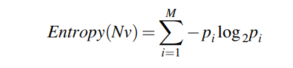
Where:
- Entropy(Nv) is the entropy of the set S.
- p(i) represents the proportion of data points belonging to a particular class or category i.
Now, let's calculate the entropy for our example dataset:
Entropy(S) = - [(40/100) * log2(40/100) + (30/100) * log2(30/100) + (30/100) * log2(30/100)]
Entropy(S) = - [(0.4 * log2(0.4)) + (0.3 * log2(0.3)) + (0.3 * log2(0.3))]
Entropy(S) ≈ - [(-0.528) + (-0.521) + (-0.521)]
Entropy(S) ≈ - (-1.570)
Entropy(S) ≈ 1.570
The entropy value for this dataset is approximately 1.570. But what does this value signify?
Entropy ranges from 0 to 1. A value of 0 indicates complete order or certainty, where all the data points belong to the same class. On the other hand, a value of 1 indicates complete
disorder or randomness, where the data points are evenly distributed across different classes.
A branch with an entropy of zero is a leaf node, whereas a branch with an entropy greater than zero requires additional splitting, according to ID3.
In our example, the entropy value of approximately 1.570 indicates a moderate level of disorder or randomness. The animals are distributed among different colors,
but there is no dominant color.
Now, let's consider another example where all the animals in the dataset are of the same color. Suppose we have 100 red animals. In this case, the entropy calculation would be as follows:
Entropy(S) = - [(100/100) * log2(100/100)]
Entropy(S) = - [1 * log2(1)]
Entropy(S) = - [0]
Entropy(S) = 0
In this scenario, the entropy value is 0, indicating complete order or certainty. Since all the animals are of the same color, there is no uncertainty or randomness.
Information Gain:
Information gain is a key concept used in decision tree algorithms to determine the best feature to split the data. It measures the reduction in entropy or
uncertainty achieved by splitting the data based on a specific attribute. The attribute that yields the highest information gain is chosen as the splitting
criterion. Let's explore information gain in more detail, using an example and the relevant mathematical formula.
To calculate the information gain, we compare the entropy of the original dataset with the weighted average of the entropies of the subsets created by the attribute split.
The formula for information gain is as follows:
To calculate information gain, we need to consider the entropy of the dataset before and after the split. The formula for information gain is as follows:
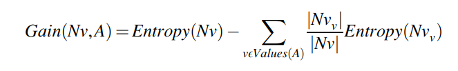
Where:
- Gain(A) represents the information gained by splitting the dataset using attribute A.
- Entropy(S) is the entropy of the original dataset S.
- Sv represents the subsets created by splitting the dataset based on attribute A.
- |Sv| and |S| denote the number of instances in subset Sv and the original dataset S, respectively.
- Entropy(Sv) represents the entropy of each subset Sv.
Let's use the previous example of animal species and their colors to illustrate the calculation of information gain.
Information gain quantifies the decrease in entropy or variance brought about by dividing the dataset into segments based on attribute A. The splitting criterion for the decision
tree is determined to be the property that optimizes information gain.
Both classification and regression decision trees employ information gain. While variance is utilized as a measure of impurity in regression, entropy is used as a measure of impurity
in classification. In both scenarios, the information gain calculation is the same, with the exception that the formula uses variance or entropy in place of entropy.
Assuming we want to determine the attribute that best separates the animals based on their colors, we can consider attributes like "age" and "habitat." Let's calculate the information
gain for both attributes:
Attribute: Age
Subsets:
Subset1 (Age <= 10): 60 animals (40 red, 20 blue, 0 green)
Subset2 (Age > 10): 40 animals (0 red, 10 blue, 30 green)
Entropy(Subsets):
Entropy(Subset1) = 0 (since all animals are red)
Entropy(Subset2) ≈ - [(0/40) * log2(0/40) + (10/40) * log2(10/40) + (30/40) * log2(30/40)]
Information Gain(Age):
Information Gain(Age) = Entropy(S) - [(60/100) * Entropy(Subset1) + (40/100) * Entropy(Subset2)]
Attribute: Habitat
Subsets:
Subset1 (Habitat = Forest): 50 animals (40 red, 10 blue, 0 green)
Subset2 (Habitat = Ocean): 30 animals (0 red, 20 blue, 10 green)
Subset3 (Habitat = Grassland): 20 animals (0 red, 0 blue, 20 green)
Entropy(Subsets):
Entropy(Subset1) ≈ - [(40/50) * log2(40/50) + (10/50) * log2(10/50) + (0/50) * log2(0/50)]
Entropy(Subset2) ≈ - [(0/30) * log2(0/30) + (20/30) * log2(20/30) + (10/30) * log2(10/30)]
Entropy(Subset3) ≈ - [(0/20) * log2(0/20) + (0/20) * log2(0/20) + (20/20) * log2(20/20)]
Information Gain(Habitat):
Information Gain(Habitat) = Entropy(S) - [(50/100) * Entropy(Subset1) + (30/100) * Entropy(Subset2) + (20/100) * Entropy(Subset3)]
By calculating the information gain for each attribute, we can determine which attribute provides the highest information gain. In this example, we compare the information gain for "age"
and "habitat" to decide which attribute is the best choice for splitting the dataset.
Please note that the calculations for entropy and information gain in this example are approximations, as the actual values were not provided. However, this example illustrates the
general process and formula used to calculate information gain.
Gini Index:
• The Gini index may be thought of as a cost function that evaluates dataset splits. It is determined by deducting one from the total of the squared
probability for each class. In contrast to information gain, which promotes smaller divisions with unique values, it favors bigger partitions and is simpler to
implement.
• The frequency with which a randomly selected element will be incorrectly detected is gauged by the Gini Index.
• When using the CART (Classification and Regression Tree) technique to create a decision tree, the Gini index is a purity or impurity indicator.
• It is preferable to have an attribute with a low Gini index than one with a high Gini value.
• It only generates binary splits, whereas the CART method generates binary splits using the Gini index.
• The Gini Index calculation formula is shown below.

In decision trees and other machine learning techniques, the Gini Index is a typical way to assess inequality or impurity in a distribution. From 0 to 1, where 0
denotes perfect equality (all values are the same), and 1 denotes perfect inequality (all values are different), the scale runs from 0 to 1.
It is computed by adding up the squared probability of each result in a distribution, then taking the sum and subtracting it from 1.
A distribution that is more homogenous or pure has a lower Gini index, whereas a distribution that is more heterogeneous or impure has a higher Gini index.
By comparing the impurity of the parent node with the weighted impurity of the child nodes, the Gini Index is used in decision trees to assess the quality of
a split.
Applications of Decision Tree
Decision tree machine learning has found wide application in various industries and domains, showcasing its effectiveness in solving complex problems. Let's look
into some real-life applications where decision tree models have proven valuable:
1. Credit Scoring:
Decision trees are extensively employed by banks and financial institutions for credit scoring. These models analyze customer data, including income, employment
history, credit history, and other relevant factors, to assess the creditworthiness of loan applicants. By evaluating the various attributes, decision trees can
determine the risk associated with granting a loan, helping lenders make informed decisions regarding loan approvals, interest rates, and credit limits.
2. Medical Diagnosis:
In the field of medicine, decision tree machine learning has significant implications for diagnosing diseases. By analyzing patient symptoms, medical history, and
test results, decision trees can assist doctors in making accurate diagnoses and recommending suitable treatment plans. The decision tree model considers various
symptoms and medical indicators to classify patients into different disease categories, aiding physicians in delivering prompt and targeted care.
3. Customer Churn Prediction:
Decision tree models are valuable for predicting customer churn in the realm of customer relationship management. By examining customer demographics, purchase history,
engagement metrics, and other relevant data, decision trees can identify patterns and factors that contribute to customer attrition. By identifying customers who are
likely to churn, businesses can take proactive measures to retain them, such as targeted marketing campaigns, personalized offers, or improved customer service.
4. Fault Diagnosis in Engineering:
Decision trees find extensive use in engineering applications, particularly in diagnosing faults in complex systems. By analyzing sensor data, system parameters,
and historical performance data, decision trees can pinpoint the root causes of faults or anomalies in machinery or industrial processes. This information enables
engineers to take appropriate actions, such as maintenance, repairs, or adjustments, to ensure the reliability, safety, and optimal functioning of the system.
These are just a few examples highlighting the practical applications of decision tree machine learning. The flexibility, interpretability, and ease of understanding
of decision trees make them suitable for a wide range of domains, where actionable insights and decision-making based on complex data patterns are essential.
Decision tree machine learning algorithms provide valuable decision-making capabilities, allowing businesses and professionals to make data-driven choices in various
fields, leading to improved efficiency, accuracy, and informed decision-making.
Advantages of decision trees in machine learning
The use of decision trees in machine learning is increasingly common. Because it visualizes the decision-making process, the resulting decision tree is simple to
comprehend. This simplifies the process of describing a model's output to stakeholders that lack specialized data analytics understanding. The model and data are
shown in a way that non-specialist stakeholders can access and comprehend, making the data available to many business teams. Thus, it is easy to comprehend the model's
logic or reasoning. This is an obvious advantage for the usage of decision trees in machine learning as explainability can be a barrier to adoption of machine learning
inside organizations.
The tree structure is one of the quickest ways to find relevant variables and links between two or more variables because of how easily it can be represented in a
flowchart. The decision tree may be used to find the most important factors in an issue that has hundreds of variables. They are also seen to be simple to comprehend,
especially by those without analytical training. Because of the visual output, statistical expertise is not required. The connections between the variables are
typically clear.
Decision-tree advantages include:
• easy to comprehend and interpret. Visualizing trees is possible.
• little data preparation is necessary. Data normalization, the creation of dummy variables, and the elimination of blank values are frequently necessary for other
procedures. The module does not, however, handle missing values.
• As more data points are utilized to train the tree, the cost of utilizing it to forecast data increases exponentially.
• capable of working with both category and numerical data. Categorical variables are not currently supported by the Scikit-Learn implementation. Other methods are
often focused on evaluating datasets with just one kind of variable.
• Capable of dealing with multi-output problems.
• using the white box model. Boolean logic makes it simple to describe a condition if it can be observed in a model for a specific circumstance. Results may be more
challenging to interpret in a black box model, such as an artificial neural network.
• It is possible to use statistical tests to verify a model. This enables the model's dependability to be taken into account.
• performs well even if the underlying model from which the data were created slightly violates some of its basic assumptions.
Disadvantages of decision trees in machine learning
The problem of overfitting is one of the key disadvantages of utilizing decision trees in machine learning. Machine learning models strive to attain a trustworthy
level of generalization such that, once deployed, the model can reliably interpret unknown input. When a model is overfitted to the training data, it may lose
accuracy when dealing with fresh data or forecasting future events.
Decision trees frequently develop into highly complicated and large structures, which can lead to overfitting as a serious problem. Pruning is a necessary step in
decision tree refinement because it prevents overfitting. When a tree is pruned, branches and nodes that are unrelated to the model's objectives or that don't add
any new information are removed.
• Decision-tree learners can produce too complicated trees that do not generalize effectively. Overfitting is the term for this. To prevent this issue,
mechanisms like pruning, defining the minimum amount of samples needed at a leaf node, or establishing the maximum depth of the tree are required.
• Because even slight changes in the data might produce an entirely different tree, decision trees can be unstable. The solution to this issue is to employ decision
trees as part of an ensemble.
• Decision tree predictions are piecewise constant approximations rather than smooth or continuous predictions. They therefore
struggle with extrapolation.
• It is well known that learning an optimum decision tree under various conditions of optimality, even for straightforward notions, is an NP-complete issue
. Because each node makes judgments that are locally optimum, heuristic algorithms like the greedy algorithm serve as the foundation for practical decision-tree
learning algorithms. Such algorithms cannot promise to deliver the decision tree that is globally optimum. Multi-tree training in an ensemble learner with replacement
sampling for the features and samples can help to reduce this.
• Certain topics, like XOR, parity, or multiplexer difficulties, are challenging to understand because decision trees do not simply describe them.
• If some classes predominate, decision tree learners will produce biased trees. Therefore, before fitting the dataset to the decision tree, it is advised to
balance the dataset.
How to avoid Overfitting in Decision Trees?
The usual difficulty with decision trees is that they fit a lot, especially in tables with many columns. The training data set may appear to have been remembered by
the tree at times. A decision tree will provide 100% accuracy on the training data set if no limits are placed since, in the worst scenario, it will produce one leaf
for each observation. As a result, this influences the precision of predictions for samples that are not included in the training set.
Overfitting is a common challenge in decision tree models, where the model becomes too complex and specific to the training data, resulting in poor generalization
to unseen data. To avoid or counter overfitting in decision trees, two effective techniques are pruning and using random forests.
1. Pruning Decision Trees:
Pruning is a technique used to reduce the complexity of a decision tree by removing unnecessary branches and nodes. It helps prevent overfitting and improves the model's ability to
generalize to new data. Two popular pruning methods are pre-pruning and post-pruning.
• Pre-pruning: In pre-pruning, the decision tree is grown by setting constraints on the tree's size and depth during the learning process. Common pre-pruning techniques include:
- Setting a maximum depth for the tree: By limiting the depth of the tree, it prevents the model from becoming too complex and overfitting.
- Setting a minimum number of samples required to split a node: This ensures that a node is only split if it contains a minimum number of samples, preventing overly specific splits based on a few observations.
- Setting a maximum number of leaf nodes: Limiting the number of leaf nodes restricts the model's complexity and encourages generalization.
• Post-pruning: In post-pruning, the decision tree is grown to its maximum size and then pruned by removing branches that do not significantly improve the model's performance on
validation data. Common post-pruning techniques include:
- Cost complexity pruning (also known as alpha pruning or weakest link pruning): This method assigns a cost parameter to each subtree and selects the subtree with the minimum cost. The
cost is determined by considering the model's accuracy and complexity.
- Reduced error pruning: This approach evaluates the impact of pruning a node by comparing the error rate before and after pruning. If the pruning leads to a decrease in error rate, the
subtree is removed.
2. Random Forest:
Random Forest is an ensemble learning method that utilizes multiple decision trees to make predictions. It helps mitigate overfitting by combining the predictions of several trees and
reducing individual tree biases. Here's how it works:
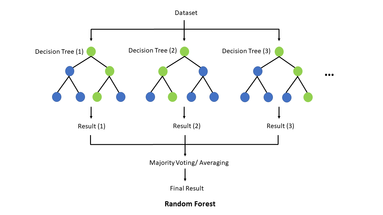
- Randomly select subsets of the training data with replacement (bootstrapping).
- Build a decision tree on each subset with a random selection of features.
- Predict the outcome by aggregating the predictions of all the trees (e.g., majority voting for classification or averaging for regression).
Random Forest improves generalization by reducing the impact of individual decision trees that may overfit the training data. By averaging predictions from multiple trees, it reduces
bias and variance, leading to better overall performance on unseen data.
Example:
Let's consider a scenario where we have a decision tree model for classifying emails as spam or not spam based on various features. If the model is overfitting, it may create complex
branches and nodes that memorize the training data, leading to poor performance on new email samples.
To counter overfitting, we can apply pruning techniques. For instance, we can set a maximum depth limit for the tree, such as 5 levels. This constraint prevents the tree from becoming
overly complex and improves generalization. Additionally, we can use cost complexity pruning, which assigns costs to subtrees based on their performance on validation data, and prunes
subtrees with higher costs.
Alternatively, we can employ a random forest approach. We create an ensemble of decision trees, each trained on a random subset of the training data and a random selection of features.
By aggregating the predictions of multiple trees, we can achieve better accuracy and reduce overfitting.
By using pruning techniques or employing random forest, we can effectively counter overfitting in decision tree models and improve their generalization capabilities to unseen data.
Conclusions
In conclusion, decision tree machine learning is a potent method that may simplify the difficulties of data processing and facilitate efficient decision-making.
It is a useful tool in many disciplines due to its interpretability, capacity to handle nonlinear connections, and feature selection skills. You may use decision trees
to get important insights from your data by comprehending how they function and how they are used.
Powerful methods for data classification and assessing the costs, risks, and possible rewards of ideas are decision tree algorithms. You may use a decision tree to
make bias-free decisions in a methodical, fact-based manner. The outputs offer choices in a manner that is simple to understand, making them applicable in a variety
of settings.
Good luck and happy learning!